Introduction
In this tutorial you will learn about dimensionality reduction techniques by using Cloudera Machine Learning (CML); an experience on Cloudera Data Platform (CDP). Dimensionality reduction techniques help in reducing the number of dimensions of data and help a model to perform well by choosing only important features required for training. By removing redundant features model size can be decreased while model training speed can be improved. Dimensionality reduction techniques also help in visualizing high dimensional data.
In this tutorial we’ll cover three commonly used dimensionality reduction techniques such as Principal Component Analysis (PCA), t-Distributed Stochastic Neighbor Embedding (t-SNE), and Uniform Manifold Approximation and Projection (UMAP). We’ll build, deploy, monitor these models to demonstrate the working of these techniques on MNIST digit recognition dataset using Cloudera Machine Learning (CML).
Prerequisites
To better understand this tutorial, you should have a basic knowledge of statistics, linear algebra and scikit-learn
Outline
Dimensionality Reduction Techniques Overview (PCA, TSNE, UMAP)
What is Dimensionality Reduction?
Data collection rate has significantly increased in recent years. As data generation and collection keeps increasing, understanding visualizing and drawing inferences from data becomes more challenging. For example, visualizing two-dimensional data with features X, Y can be done easily using a scatter plot whereas if you have data with 5 dimensions it is impossible to visualize that data using traditional techniques. Hence, dimensionality reduction helps in solving this issue. Below are some benefits applying dimensionality reduction to a dataset.
- Reducing the number of dimensions leads to less computation and helps a model to perform well by choosing only important features required for training and removes redundant features thereby decreasing the storage and increasing the computation speed.
- Dimensionality reduction helps in visualization of data especially when the data is in higher dimensions.
Common Dimensionality Reduction Techniques
In this section we will be discussing three common dimensionality reduction techniques that are widely used and implemented using python and scikit-learn.
Principal Component Analysis (PCA)
PCA is a technique that helps in extracting new sets of variables from an existing set of variables that are known as principal components. A principal component is nothing more but a linear combination of the original variables. Principal components play a key role in PCA by allowing data to be projected into lower dimensions from higher dimensional space. For example, let’s consider a dataset with 10 dimensions being reduced to three dimensions using PCA. The three dimensions are the principal components of a dataset; they represent most of the information about that dataset. The first principal component explains maximum variance in the dataset, the second explains the remaining variance unexplained by the first principal component, and the third principal component explains variance unexplained by first and second components and so on.
t-Distributed Stochastic Neighbor Embedding (t-SNE)
We have learned that PCA is a good choice for dimensionality reduction and visualization of large linear datasets. For non-linear datasets, t- Distributed Stochastic Neighbor Embedding (t-SNE) is a good technique. This algorithm has the capability to calculate similarity of points in both low and high dimensional space. The algorithm calculates the probability of similarity of points in high-dimensional space and also calculates the similarity of points in the corresponding low-dimensional space. It then tries to minimize the difference between the similarities in both low and high dimensional space for a good representation of data points in lower-dimensional space. t-SNE helps map the multidimensional space and make attempts to find patterns in the data by identifying the clusters based on similarity of the data points to multiple features to project into lower dimensional space.
Uniform Manifold Approximation and Projection (UMAP)
Although t-SNE works well on large datasets, it is neither efficient in computation time nor in meaningfully representing large scale information. UMAP is another technique that has the capability to preserve the local and global structure of data with less computation time.
Unlike t-SNE, which uses Euclidean distance metric to calculate the similarities, UMAP uses k-nearest neighbor approach (unsupervised machine learning). First, it calculates the distance between the points in the high dimensional space. Second, it projects them onto low dimensional space. Third, it calculates the distance between the points in low dimensional space.
Model Creation and Deployment using Cloudera Machine Learning
This section describes an example of how to create and deploy a model using CML.
Using CML, you can deploy a Machine Learning model via a REST API. This API will accept input variables and return a prediction. For the purpose of this tutorial, we are going to create a model that will demonstrate the concepts of PCA, TSNE and UMAP dimensionality reduction techniques using scikit-learn. To run this project, you will need to set up your environment. Follow the steps below.
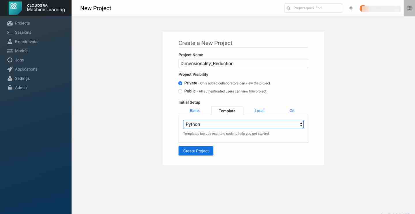
First, create a new project. Note that models are always created within the context of a project. Name your project and pick python as your template to run the code.
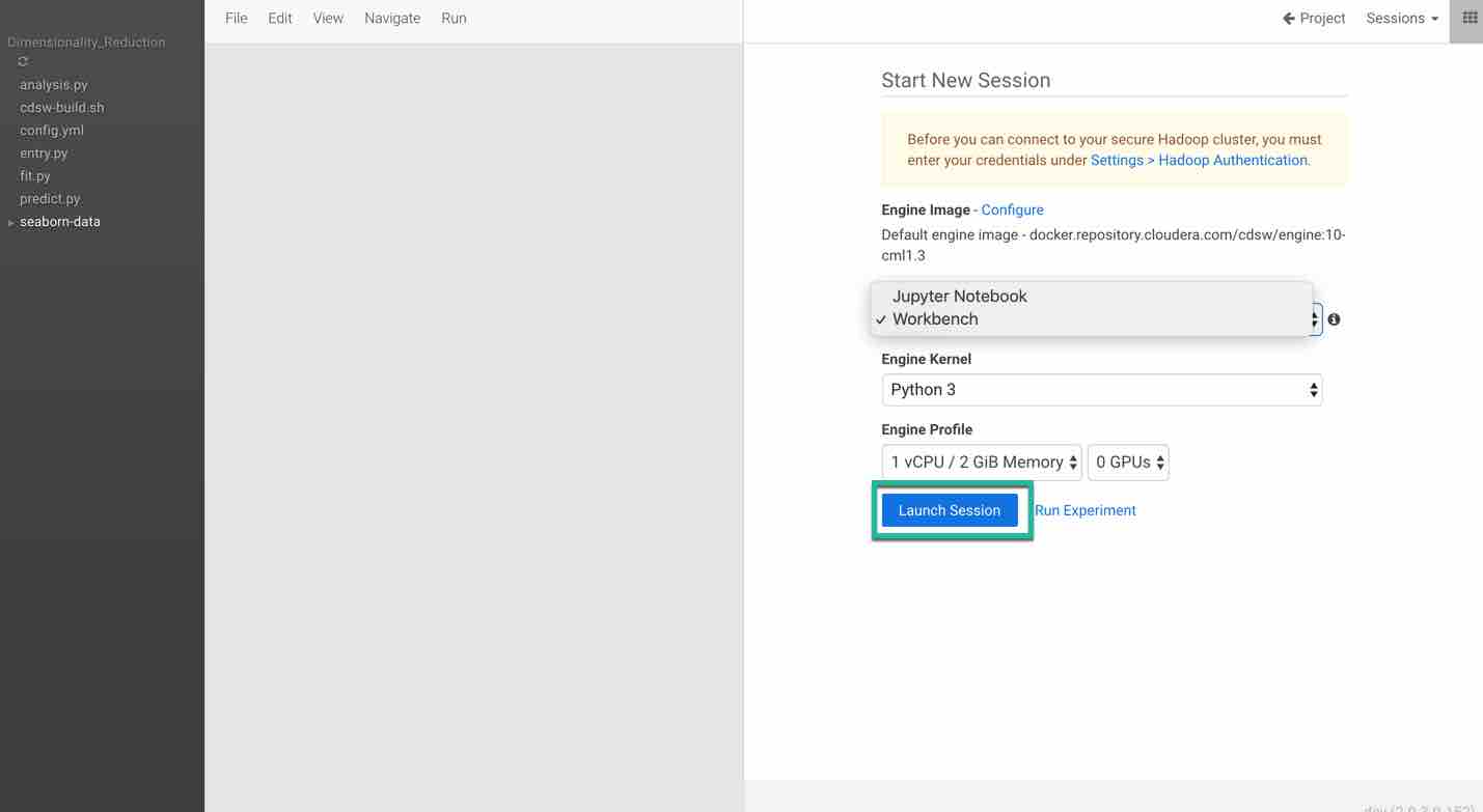
Click Open Workbench and launch a new Python 3 session. You have flexibility to choose either a Jupyter notebook or a workbench. In this tutorial we will import the code into the workbench and run the code.
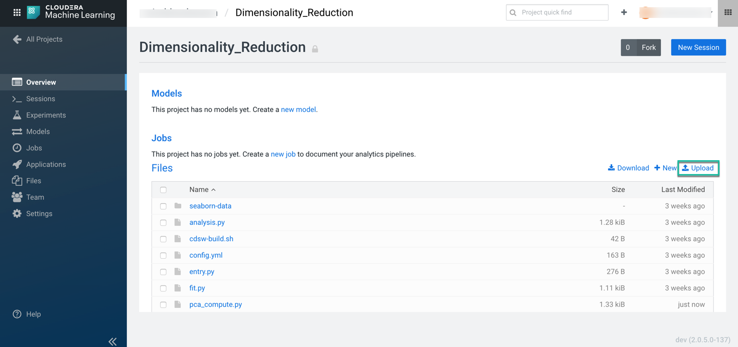
Next, download the code snippet and unzip it on your local machine. Upload pca_compute.py file using the upload option in the CML project overview page to execute the code and visualize the results.
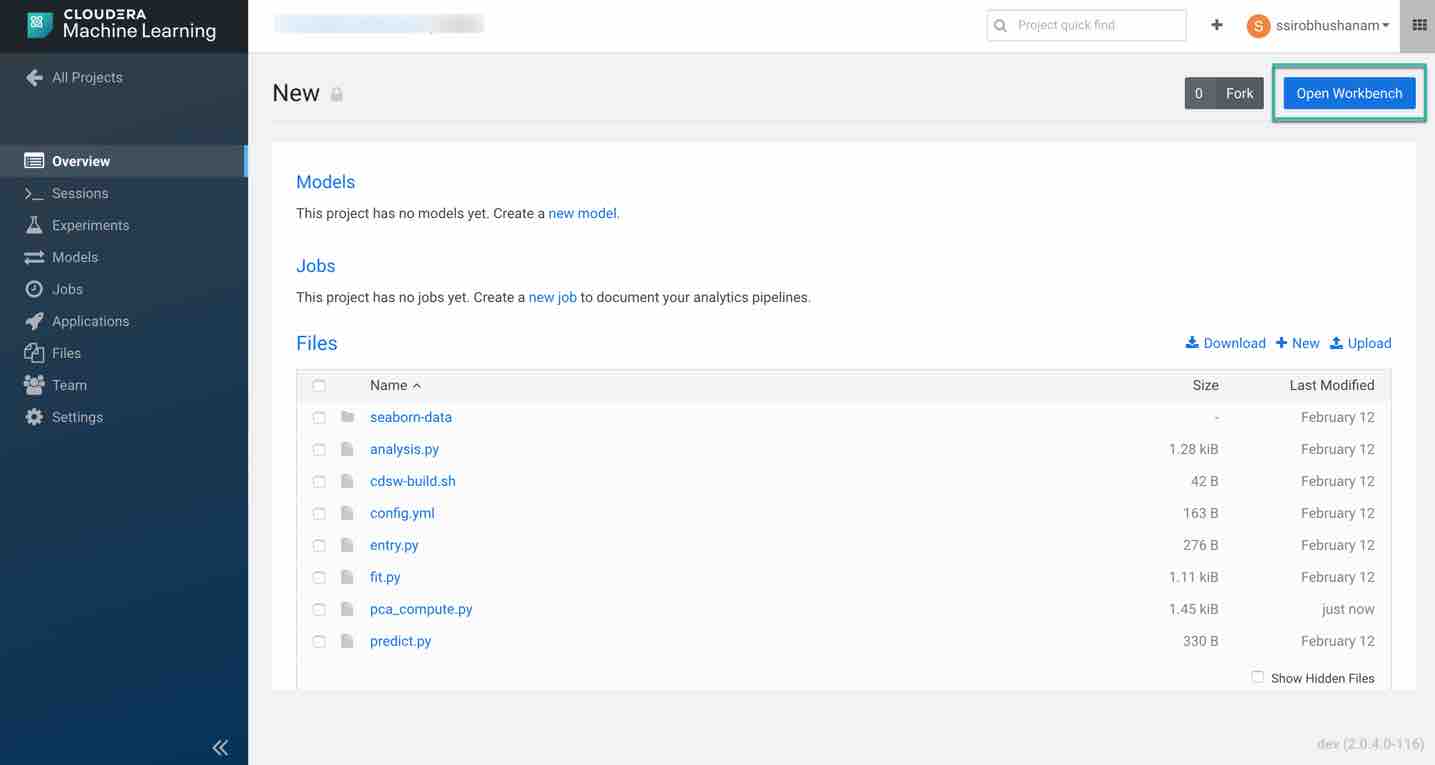
Once the file is uploaded successfully, provision your workspace by clicking on Open Workbench in the top right of the overview page.
Choose the desired system specifications. For this tutorial, we are using the following specifications:
- Editor: Workbench (you can also choose Jupyter Notebook to run the code)
- Engine Kernel: Python3
- Engine Profile: 1 CPU/ 2 GB Memory
Click on Launch Session and select pca_compute.py in the left pane. The code in the workspace should look as below.
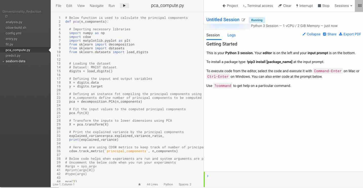
The main purpose of this code snippet is to calculate the principal components for the dataset. We defined a function named pca with arguments n_components, which are the number of principal components to be calculated. When you execute this code, you can see three principal components for the dataset. Once you have the principal components, you can find the explained_variance. It will provide you with the amount of information or variance each principal component holds after projecting the data to a lower dimensional subspace.
Next, run the code snippet. Your output should look as follows:

From the above output, you can observe that the principal component one holds 14.8% of the information while the principal component two holds only 13.6% of the information, and principal component three holds about 11%. Also, note that by projecting twenty-dimensional data to a three-dimensional data over 60% of information was lost.
Running Model Experiments using CML
As an example, you can run the pca_compute.py script to launch the experiment which accepts n_components as arguments and prints the explained_variance of the principal components. You can initially test your script to avoid any errors during running your experiments. You can also launch a session to simultaneously test code changes on the interactive console as you launch new experiments.
To test the script, launch a Python session and run the following command from the workbench command prompt:
!python pca_compute.py 5

Now to run the experiment click on Run > Run Experiment if you are already on an active session. Fill out the fields:
- Script: Provide the script to run the experiment, here we are using pca_compute.py
- Arguments: This python script accepts n_components as arguments. Enter a value in this field
- Engine Kernel: For this script you need to choose python3
- Engine Profile: You can leave this as default or you can choose your configuration. For this script we are using 1 CPU/ 2 GB memory with no GPU as this is very simple script to run
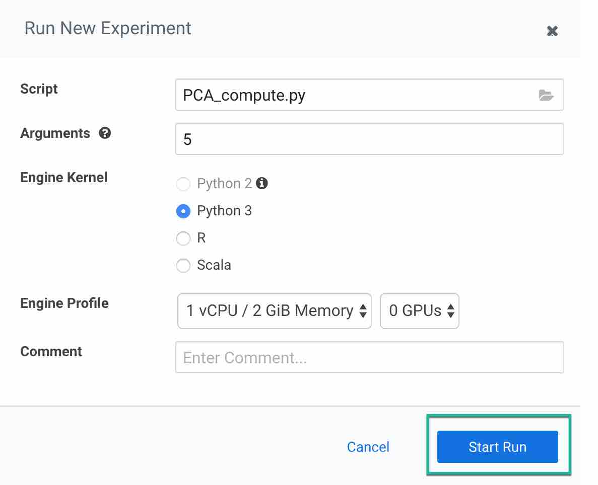
Then click on Start Run to run the experiment and observe the results.
To track progress for the run, go back to the project overview. On the left navigation bar click Experiments. You should see the experiment you've just run at the top of the list.
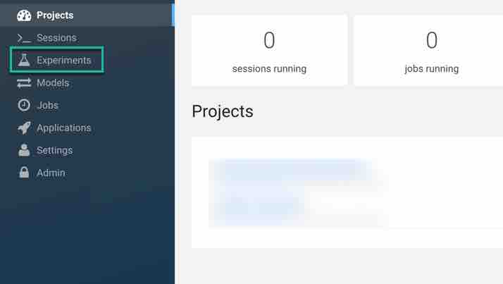
Click on the Run ID to view an overview for each individual run. Then click Build. On this Build tab you can see real time progress as CML builds the Docker image for this experiment. This allows you to debug any errors that might occur during the build stage.

Once the Docker image is ready, the run will begin execution. You can track progress for this stage by going to the Session tab. You can also check for errors in the session to understand the run time errors encountered during the experiment.
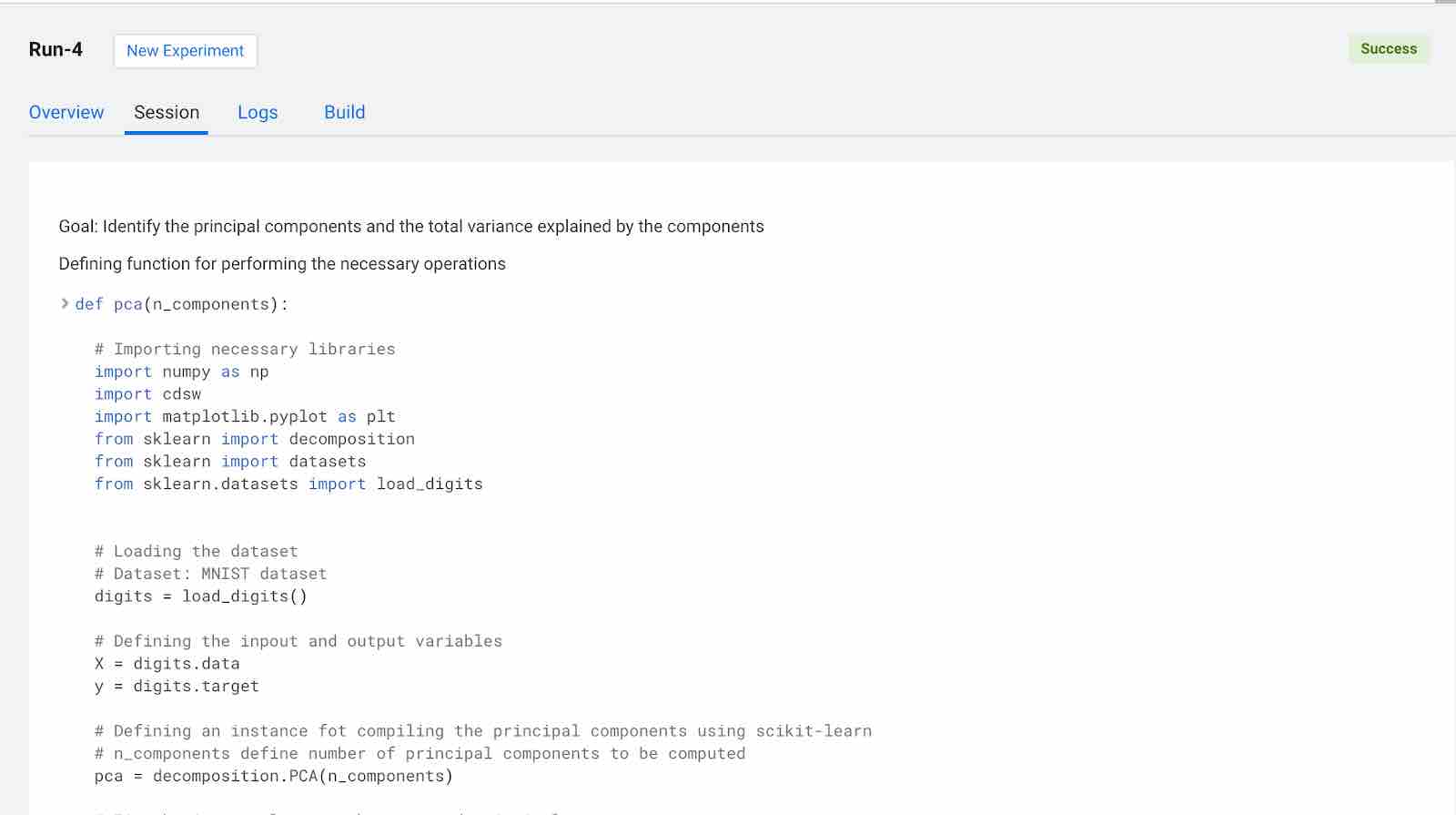
When conducting experiments in real time we are always curious to keep track of metrics useful for tracking the performance of the model. CML includes some built-in functions that you can use to compare experiments and save any files from your experiments using the CML library.
As an example, using the pca_compute.py script we will include a metric called principal components to track the number of principal components being calculated by the script. In order to perform this, the script imported the CML library and added the following line to the script.
Deploying Model using CML
This section gives information about deploying the model using CML. We are using the same script to deploy the model.
Navigate to the project overview > Models page.
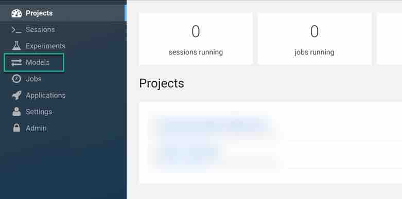
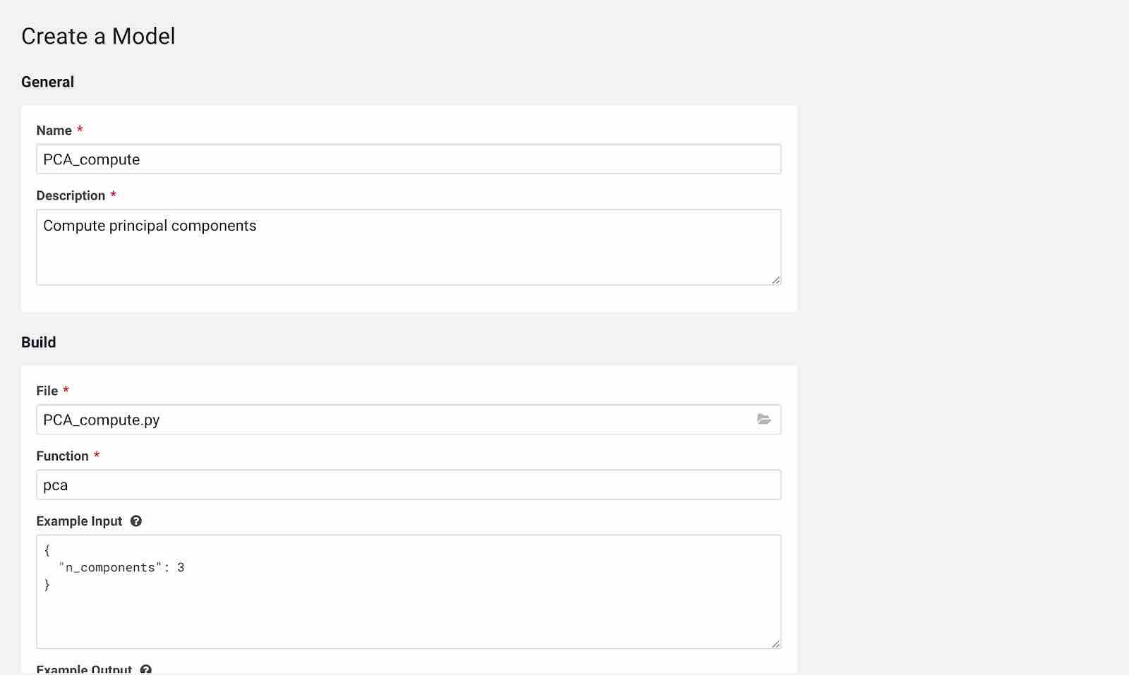
Click New Model and fill out the fields as shown below. Make sure you use the Python 3 kernel. For example, here we are using pca_compute.py script and example input would be the n_components written in JSON format. You have flexibility to choose the engine profile and GPU capability if needed and CML also provides an option to choose replicas for your model which helps in avoiding single point of failure when your models are in production.
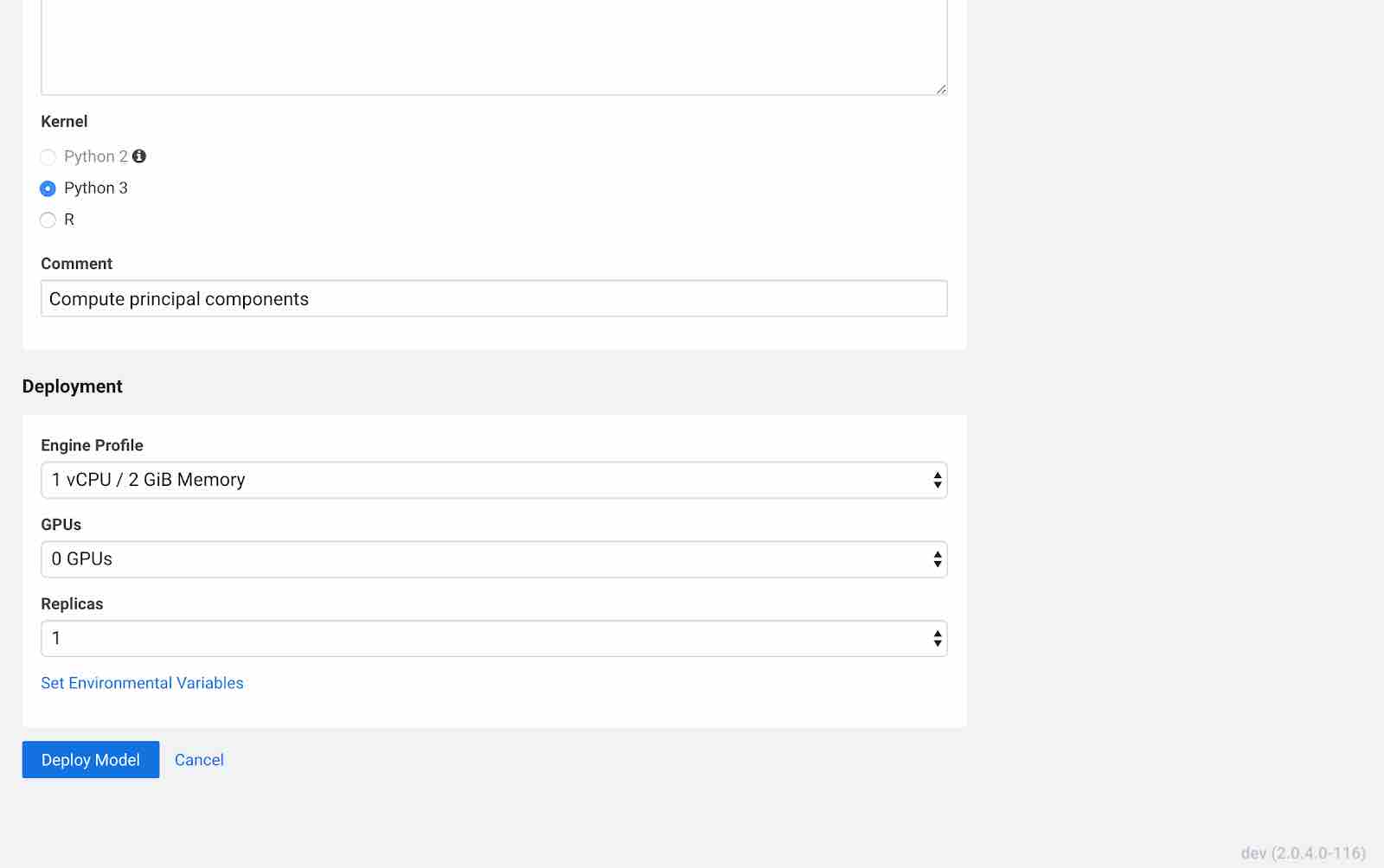
Click Deploy Model. Click on the model to go to its overview page. As the model builds you can track progress on the Build page. Once deployed, you can see the replicas deployed on the Monitoring page.
Model successfully deployed

Check Builds tab to track the progress of the model

Monitoring tab provides information about your model. You can see replica information, processed, failure, status, errors and more.

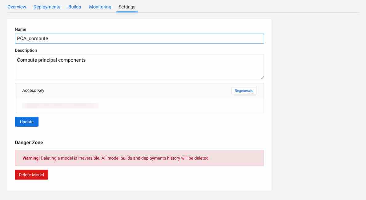
When you click on settings, you also have an option to delete your model.
Data Visualization using Dimensionality Reduction Techniques
As we have already discussed how PCA, T-SNE, UMAP help in visualizing a dataset. Let us now use the script dimensionality_reduction_viz.py to build the models and visualize the results.
Similar to Section 2, import the code snippet dimensionality_reduction_viz.py into the CML workspace.
First, select the pca function that is used to calculate two principal components and visualize the MNIST dataset using the two principal components. Call the function using the following command pca() to plot the results. Steps followed by the function to print the results are as follows:
- Import all the necessary libraries: Here we are using numpy, sklearn decomposition, sklearn datasets, sklearn load_digits dataset, pandas, matplotlib and seaborn for visualization, pca for building pca model on the dataset.
Note: Before execution of the code make sure to install sklearn, umap, seaborn, matplotlib, numpy
- Load the dataset using scikit-learn load_digits() function
- Feed the features into X and target into y variables
- Instantiate pca with arguments as n_components(here we are using 2)
- Fit the pca embedding on the dataset using fit_transform method
- Plot the visualization of the embedding for two principal components obtained
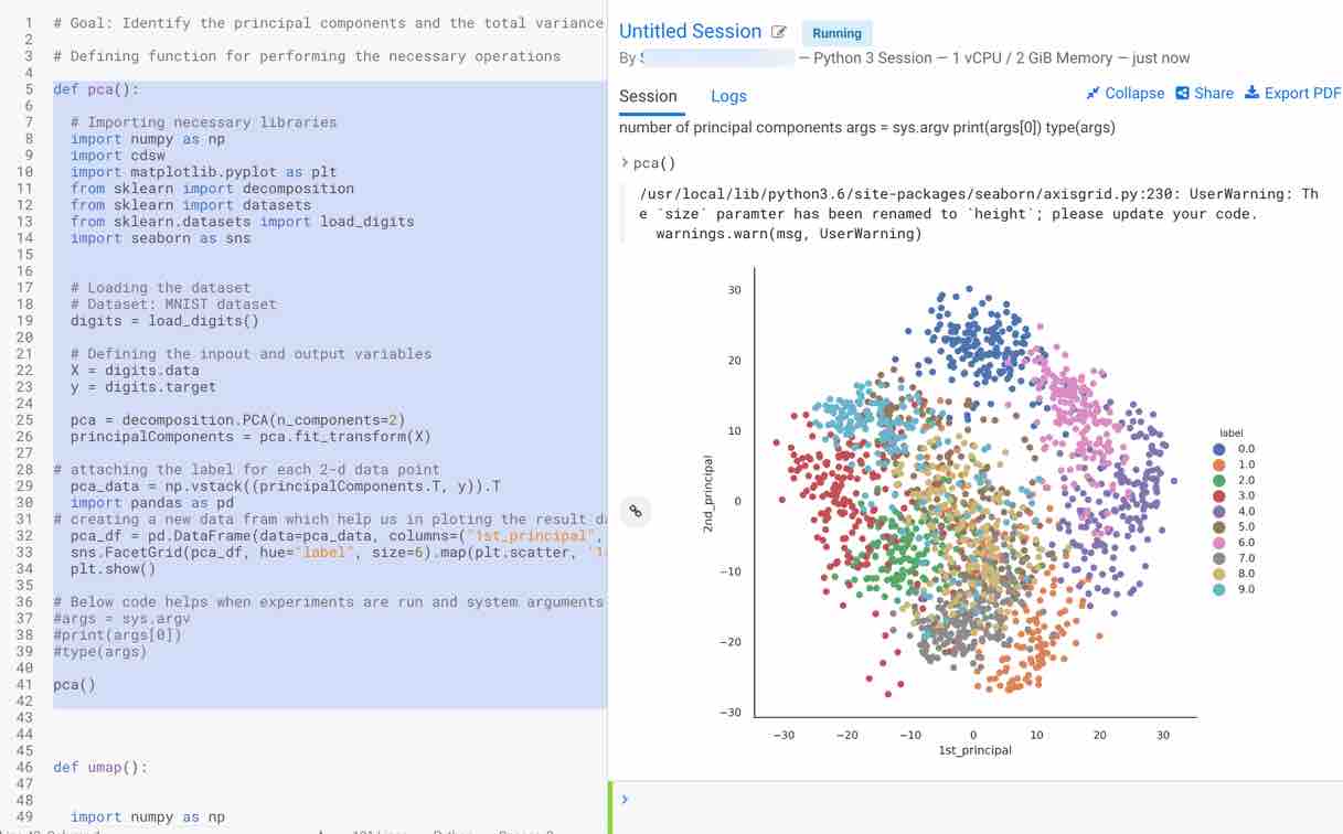
As you can observe, it is more cluttered and the data which is being sent to the algorithm is not linear. Principal components, which are linear combinations of existing features, are not so efficient in interpreting complex polynomial relationships between features due to their linearity. Hence, nonlinear approaches like UMAP and TSNE can be useful in this scenario.
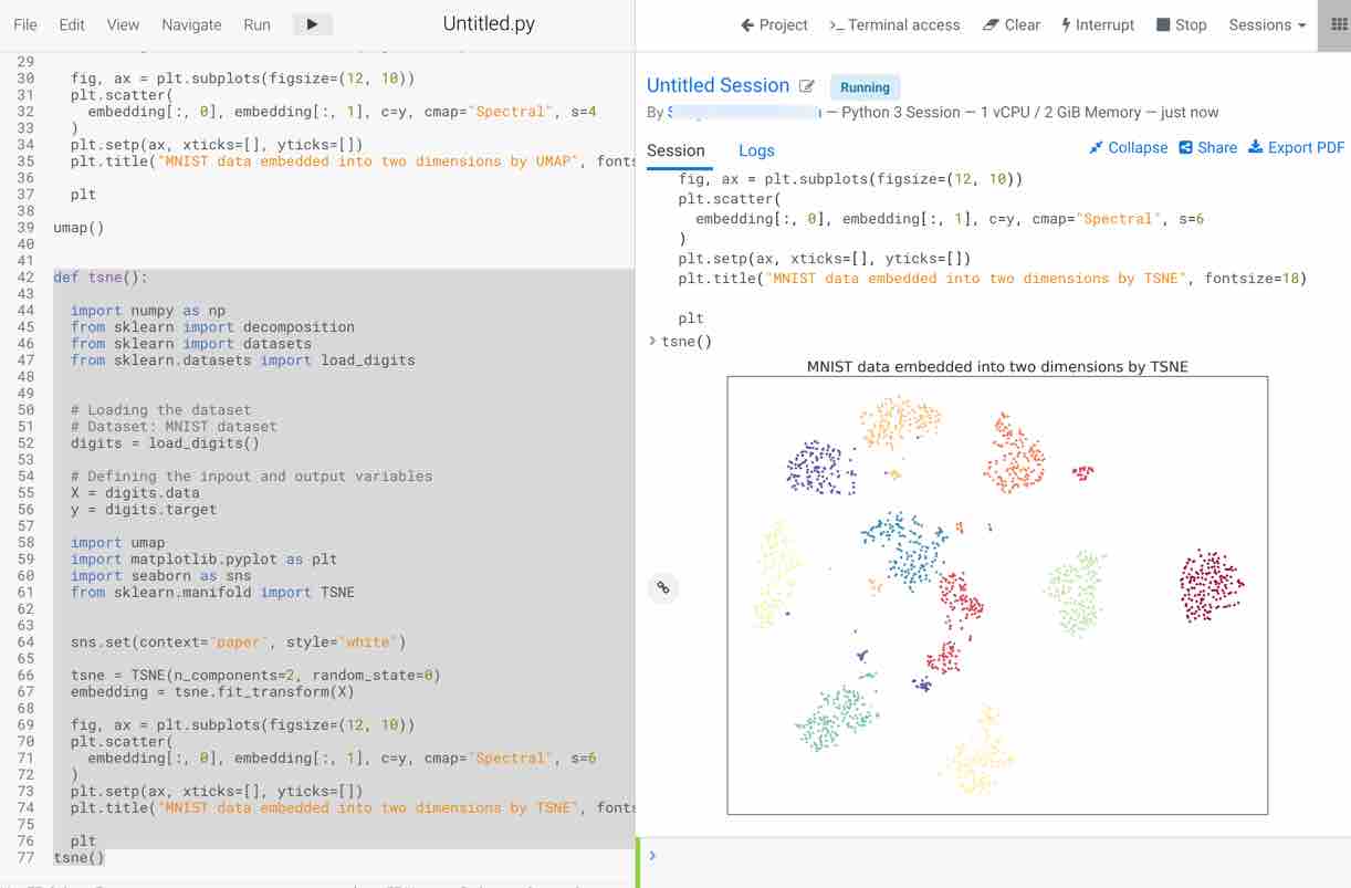
If the relationship between the variables is nonlinear PCA performs poorly. In order to deal with nonlinear data, advanced techniques like TSNE and UMAP (discussed in detail in Section 1) are more useful. Let’s now run the t-SNE function to visualize the two principal components. Steps followed by the function to print the results are as follows:
- Import all the necessary libraries: Here we are using numpy, sklearn decomposition, sklearn datasets, sklearn load_digits dataset, matplotlib and seaborn for visualization, t-sne for building t-sne model on the dataset.
Note: Before execution of the code make sure to install sklearn, umap, seaborn, matplotlib, numpy
- Load the dataset using scikit-learn load_digits() function
- Feed the features into X and target into y variables
- Instantiate t-SNE with arguments as n_components (here we are using 2) and random_state =0 which allows reproducing the results
- Fit the t-SNE embedding on the dataset using fit_transform method
- Plot the visualization of the embedding for two principal components obtained
- The plot appears on the right-hand side. You should notice that this method takes some time to execute but visualizes the data in a more efficient way compared to PCA
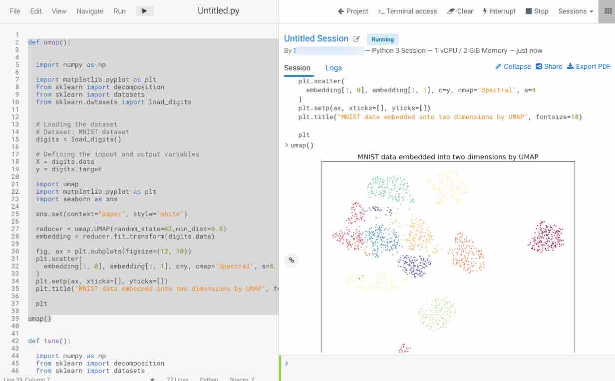
Next, select the umap function to run the code and visualize the result. Steps followed by the function to print the results are as follows
- Import all the necessary libraries: Here we are using numpy, sklearn decomposition, sklearn datasets, sklearn load_digits dataset, matplotlib and seaborn for visualization, umap for building umap model on the dataset
Note: Before execution of the code make sure to install sklearn, umap, seaborn, matplotlib, numpy
- Load the dataset using scikit-learn load_digits() function
- Feed the features into X and target into y variables
- Instantiate umap with arguments as min_dist(here we are using 0.8) and random_state =42 which allows reproducing the results
- Fit the umap embedding on the dataset using fit_transform method
- Plot the visualization of the embedding for two principal components obtained
- The plot appears on the right-hand side, as you can observe this method is faster in execution and visualizes the data in a more efficient way compared to PCA and t-SNE.
Summary
Great Job! You have learned concepts behind dimensionality reduction techniques using Cloudera Machine Learning and how CML can be used for delivering end-to-end machine learning, from model development to model deployment.
Further Reading
- Learn more about Machine Learning/Deep Learning:
- Cloudera Machine Learning Documentation

