Tuning Spark Applications
This topic describes various aspects in tuning Spark applications. During tuning you should monitor application behavior to determine the effect of tuning actions.
For information on monitoring Spark applications, see Monitoring Spark Applications.
Continue reading:
Shuffle Overview
A Spark dataset comprises a fixed number of partitions, each of which comprises a number of records. For the datasets returned by narrow transformations, such as map and filter, the records required to compute the records in a single partition reside in a single partition in the parent dataset. Each object is only dependent on a single object in the parent. Operations such as coalesce can result in a task processing multiple input partitions, but the transformation is still considered narrow because the input records used to compute any single output record can still only reside in a limited subset of the partitions.
Spark also supports transformations with wide dependencies, such as groupByKey and reduceByKey. In these dependencies, the data required to compute the records in a single partition can reside in many partitions of the parent dataset. To perform these transformations, all of the tuples with the same key must end up in the same partition, processed by the same task. To satisfy this requirement, Spark performs a shuffle, which transfers data around the cluster and results in a new stage with a new set of partitions.
For example, consider the following code:
sc.textFile("someFile.txt").map(mapFunc).flatMap(flatMapFunc).filter(filterFunc).count()
It runs a single action, count, which depends on a sequence of three transformations on a dataset derived from a text file. This code runs in a single stage, because none of the outputs of these three transformations depend on data that comes from different partitions than their inputs.
In contrast, this Scala code finds how many times each character appears in all the words that appear more than 1,000 times in a text file:
val tokenized = sc.textFile(args(0)).flatMap(_.split(' '))
val wordCounts = tokenized.map((_, 1)).reduceByKey(_ + _)
val filtered = wordCounts.filter(_._2 >= 1000)
val charCounts = filtered.flatMap(_._1.toCharArray).map((_, 1)).reduceByKey(_ + _)
charCounts.collect()
This example has three stages. The two reduceByKey transformations each trigger stage boundaries, because computing their outputs requires repartitioning the data by keys.
A final example is this more complicated transformation graph, which includes a join transformation with multiple dependencies:
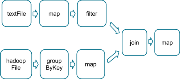
The pink boxes show the resulting stage graph used to run it:
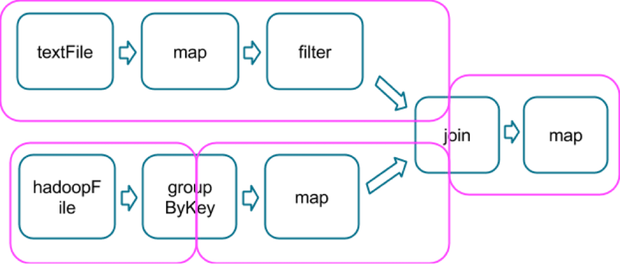
At each stage boundary, data is written to disk by tasks in the parent stages and then fetched over the network by tasks in the child stage. Because they incur high disk and network I/O, stage boundaries can be expensive and should be avoided when possible. The number of data partitions in a parent stage may be different than the number of partitions in a child stage. Transformations that can trigger a stage boundary typically accept a numPartitions argument, which specifies into how many partitions to split the data in the child stage. Just as the number of reducers is an important parameter in MapReduce jobs, the number of partitions at stage boundaries can determine an application's performance. Tuning the Number of Partitions describes how to tune this number.
Choosing Transformations to Minimize Shuffles
You can usually choose from many arrangements of actions and transformations that produce the same results. However, not all these arrangements result in the same performance. Avoiding common pitfalls and picking the right arrangement can significantly improve an application's performance.
When choosing an arrangement of transformations, minimize the number of shuffles and the amount of data shuffled. Shuffles are expensive operations; all shuffle data must be written to disk and then transferred over the network. repartition , join, cogroup, and any of the *By or *ByKey transformations can result in shuffles. Not all these transformations are equal, however, and you should avoid the following patterns:
- groupByKey when performing an associative reductive operation. For example, rdd.groupByKey().mapValues(_.sum) produces the same result as rdd.reduceByKey(_ + _). However, the former transfers the entire dataset across the network, while the latter computes local sums for each key in each partition and combines those local sums into larger sums after shuffling.
- reduceByKey when the input and output value types are different. For example, consider writing a transformation that finds all the
unique strings corresponding to each key. You could use map to transform each element into a Set and then combine the Sets with reduceByKey:
rdd.map(kv => (kv._1, new Set[String]() + kv._2)).reduceByKey(_ ++ _)
This results in unnecessary object creation because a new set must be allocated for each record.
Instead, use aggregateByKey, which performs the map-side aggregation more efficiently:
val zero = new collection.mutable.Set[String]()
rdd.aggregateByKey(zero)((set, v) => set += v,(set1, set2) => set1 ++= set2)
- flatMap-join-groupBy. When two datasets are already grouped by key and you want to join them and keep them grouped, use cogroup. This avoids the overhead associated with unpacking and repacking the groups.
When Shuffles Do Not Occur
In some circumstances, the transformations described previously do not result in shuffles. Spark does not shuffle when a previous transformation has already partitioned the data according to the same partitioner. Consider the following flow:
rdd1 = someRdd.reduceByKey(...)
rdd2 = someOtherRdd.reduceByKey(...)
rdd3 = rdd1.join(rdd2)
Because no partitioner is passed to reduceByKey, the default partitioner is used, resulting in rdd1 and rdd2 both being hash-partitioned. These two reduceByKey transformations result in two shuffles. If the datasets have the same number of partitions, a join requires no additional shuffling. Because the datasets are partitioned identically, the set of keys in any single partition of rdd1 can only occur in a single partition of rdd2. Therefore, the contents of any single output partition of rdd3 depends only on the contents of a single partition in rdd1 and single partition in rdd2, and a third shuffle is not required.
For example, if someRdd has four partitions, someOtherRdd has two partitions, and both the reduceByKeys use three partitions, the set of tasks that run would look like this:
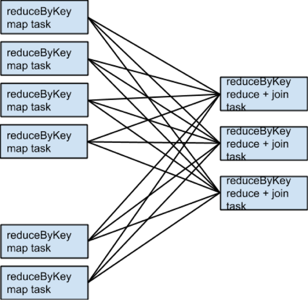
If rdd1 and rdd2 use different partitioners or use the default (hash) partitioner with different numbers of partitions, only one of the datasets (the one with the fewer number of partitions) needs to be reshuffled for the join:
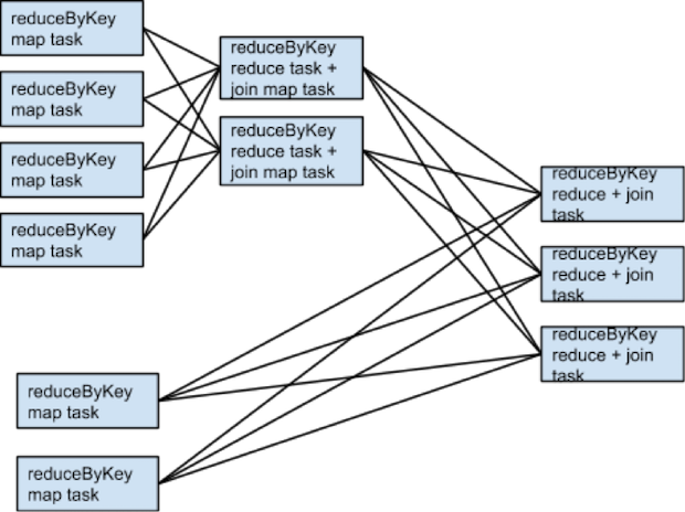
To avoid shuffles when joining two datasets, you can use broadcast variables. When one of the datasets is small enough to fit in memory in a single executor, it can be loaded into a hash table on the driver and then broadcast to every executor. A map transformation can then reference the hash table to do lookups.
When to Add a Shuffle Transformation
The rule of minimizing the number of shuffles has some exceptions.
An extra shuffle can be advantageous when it increases parallelism. For example, if your data arrives in a few large unsplittable files, the partitioning dictated by the InputFormat might place large numbers of records in each partition, while not generating enough partitions to use all available cores. In this case, invoking repartition with a high number of partitions (which triggers a shuffle) after loading the data allows the transformations that follow to use more of the cluster's CPU.
Another example arises when using the reduce or aggregate action to aggregate data into the driver. When aggregating over a high number of partitions, the computation can quickly become bottlenecked on a single thread in the driver merging all the results together. To lighten the load on the driver, first use reduceByKey or aggregateByKey to perform a round of distributed aggregation that divides the dataset into a smaller number of partitions. The values in each partition are merged with each other in parallel, before being sent to the driver for a final round of aggregation. See treeReduce and treeAggregate for examples of how to do that.
This method is especially useful when the aggregation is already grouped by a key. For example, consider an application that counts the occurrences of each word in a corpus and pulls the results into the driver as a map. One approach, which can be accomplished with the aggregate action, is to compute a local map at each partition and then merge the maps at the driver. The alternative approach, which can be accomplished with aggregateByKey, is to perform the count in a fully distributed way, and then simply collectAsMap the results to the driver.
Secondary Sort
The repartitionAndSortWithinPartitions transformation repartitions the dataset according to a partitioner and, within each resulting partition, sorts records by their keys. This transformation pushes sorting down into the shuffle machinery, where large amounts of data can be spilled efficiently and sorting can be combined with other operations.
For example, Apache Hive on Spark uses this transformation inside its join implementation. It also acts as a vital building block in the secondary sort pattern, in which you group records by key and then, when iterating over the values that correspond to a key, have them appear in a particular order. This scenario occurs in algorithms that need to group events by user and then analyze the events for each user, based on the time they occurred.
Tuning Resource Allocation
For background information on how Spark applications use the YARN cluster manager, see Running Spark Applications on YARN.
The two main resources that Spark and YARN manage are CPU and memory. Disk and network I/O affect Spark performance as well, but neither Spark nor YARN actively manage them.
Every Spark executor in an application has the same fixed number of cores and same fixed heap size. Specify the number of cores with the --executor-cores command-line flag, or by setting the spark.executor.cores property. Similarly, control the heap size with the --executor-memory flag or the spark.executor.memory property. The cores property controls the number of concurrent tasks an executor can run. For example, set --executor-cores 5 for each executor to run a maximum of five tasks at the same time. The memory property controls the amount of data Spark can cache, as well as the maximum sizes of the shuffle data structures used for grouping, aggregations, and joins.
Starting with CDH 5.5 dynamic allocation, which adds and removes executors dynamically, is enabled. To explicitly control the number of executors, you can override dynamic allocation by setting the --num-executors command-line flag or spark.executor.instances configuration property.
Consider also how the resources requested by Spark fit into resources YARN has available. The relevant YARN properties are:
- yarn.nodemanager.resource.memory-mb controls the maximum sum of memory used by the containers on each host.
- yarn.nodemanager.resource.cpu-vcores controls the maximum sum of cores used by the containers on each host.
Requesting five executor cores results in a request to YARN for five cores. The memory requested from YARN is more complex for two reasons:
- The --executor-memory/spark.executor.memory property controls the executor heap size, but executors can also use some memory off heap, for example, Java NIO direct buffers. The value of the spark.yarn.executor.memoryOverhead property is added to the executor memory to determine the full memory request to YARN for each executor. It defaults to max(384, .1 * spark.executor.memory).
- YARN may round the requested memory up slightly. The yarn.scheduler.minimum-allocation-mb and yarn.scheduler.increment-allocation-mb properties control the minimum and increment request values, respectively.
The following diagram (not to scale with defaults) shows the hierarchy of memory properties in Spark and YARN:
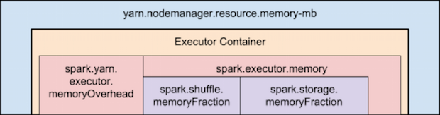
Keep the following in mind when sizing Spark executors:
- The ApplicationMaster, which is a non-executor container that can request containers from YARN, requires memory and CPU that must be accounted for. In client deployment mode, they default to 1024 MB and one core. In cluster deployment mode, the ApplicationMaster runs the driver, so consider bolstering its resources with the --driver-memory and --driver-cores flags.
- Running executors with too much memory often results in excessive garbage-collection delays. For a single executor, use 64 GB as an upper limit.
- The HDFS client has difficulty processing many concurrent threads. At most, five tasks per executor can achieve full write throughput, so keep the number of cores per executor below that number.
- Running tiny executors (with a single core and just enough memory needed to run a single task, for example) offsets the benefits of running multiple tasks in a single JVM. For example, broadcast variables must be replicated once on each executor, so many small executors results in many more copies of the data.
Resource Tuning Example
Consider a cluster with six hosts running NodeManagers, each equipped with 16 cores and 64 GB of memory.
The NodeManager capacities, yarn.nodemanager.resource.memory-mb and yarn.nodemanager.resource.cpu-vcores, should be set to 63 * 1024 = 64512 (megabytes) and 15, respectively. Avoid allocating 100% of the resources to YARN containers because the host needs some resources to run the OS and Hadoop daemons. In this case, leave one GB and one core for these system processes. Cloudera Manager accounts for these and configures these YARN properties automatically.
You might consider using --num-executors 6 --executor-cores 15 --executor-memory 63G. However, this approach does not work:
- 63 GB plus the executor memory overhead does not fit within the 63 GB capacity of the NodeManagers.
- The ApplicationMaster uses a core on one of the hosts, so there is no room for a 15-core executor on that host.
- 15 cores per executor can lead to bad HDFS I/O throughput.
Instead, use --num-executors 17 --executor-cores 5 --executor-memory 19G:
- This results in three executors on all hosts except for the one with the ApplicationMaster, which has two executors.
- --executor-memory is computed as (63/3 executors per host) = 21. 21 * 0.07 = 1.47. 21 - 1.47 ~ 19.
Tuning the Number of Partitions
Spark has limited capacity to determine optimal parallelism. Every Spark stage has a number of tasks, each of which processes data sequentially. The number of tasks per stage is the most important parameter in determining performance.
As described in Spark Execution Model, Spark groups datasets into stages. The number of tasks in a stage is the same as the number of partitions in the last dataset in the stage. The number of partitions in a dataset is the same as the number of partitions in the datasets on which it depends, with the following exceptions:
- The coalesce transformation creates a dataset with fewer partitions than its parent dataset.
- The union transformation creates a dataset with the sum of its parents' number of partitions.
- The cartesian transformation creates a dataset with the product of its parents' number of partitions.
Datasets with no parents, such as those produced by textFile or hadoopFile, have their partitions determined by the underlying MapReduce InputFormat used. Typically, there is a partition for each HDFS block being read. The number of partitions for datasets produced by parallelize are specified in the method, or spark.default.parallelism if not specified. To determine the number of partitions in an dataset, call rdd.partitions().size().
If the number of tasks is smaller than number of slots available to run them, CPU usage is suboptimal. In addition, more memory is used by any aggregation operations that occur in each task. In join, cogroup, or *ByKey operations, objects are held in in hashmaps or in-memory buffers to group or sort. join, cogroup, and groupByKey use these data structures in the tasks for the stages that are on the fetching side of the shuffles they trigger. reduceByKey and aggregateByKey use data structures in the tasks for the stages on both sides of the shuffles they trigger. If the records in these aggregation operations exceed memory, the following issues can occur:
- Holding a high number records in these data structures increases garbage collection, which can lead to pauses in computation.
- Spark spills them to disk, causing disk I/O and sorting that leads to job stalls.
To increase the number of partitions if the stage is reading from Hadoop:
- Use the repartition transformation, which triggers a shuffle.
- Configure your InputFormat to create more splits.
- Write the input data to HDFS with a smaller block size.
If the stage is receiving input from another stage, the transformation that triggered the stage boundary accepts a numPartitions argument:
val rdd2 = rdd1.reduceByKey(_ + _, numPartitions = X)
Determining the optimal value for X requires experimentation. Find the number of partitions in the parent dataset, and then multiply that by 1.5 until performance stops improving.
(spark.executor.memory * spark.shuffle.memoryFraction * spark.shuffle.safetyFraction)/
spark.executor.cores
memoryFraction and safetyFraction default to 0.2 and 0.8 respectively.
(observed shuffle write) * (observed shuffle spill memory) * (spark.executor.cores)/
(observed shuffle spill disk) * (spark.executor.memory) * (spark.shuffle.memoryFraction) * (spark.shuffle.safetyFraction)
Then, round up slightly, because too many partitions is usually better than too few.
When in doubt, err on the side of a larger number of tasks (and thus partitions). This contrasts with recommendations for MapReduce, which unlike Spark, has a high startup overhead for tasks.
Reducing the Size of Data Structures
Data flows through Spark in the form of records. A record has two representations: a deserialized Java object representation and a serialized binary representation. In general, Spark uses the deserialized representation for records in memory and the serialized representation for records stored on disk or transferred over the network. For sort-based shuffles, in-memory shuffle data is stored in serialized form.
The spark.serializer property controls the serializer used to convert between these two representations. Cloudera recommends using the Kryo serializer, org.apache.spark.serializer.KryoSerializer.
The footprint of your records in these two representations has a significant impact on Spark performance. Review the data types that are passed and look for places to reduce their size. Large deserialized objects result in Spark spilling data to disk more often and reduces the number of deserialized records Spark can cache (for example, at the MEMORY storage level). The Apache Spark tuning guide describes how to reduce the size of such objects. Large serialized objects result in greater disk and network I/O, as well as reduce the number of serialized records Spark can cache (for example, at the MEMORY_SER storage level.) Make sure to register any custom classes you use with the SparkConf#registerKryoClasses API.
Choosing Data Formats
When storing data on disk, use an extensible binary format like Avro, Parquet, Thrift, or Protobuf and store in a sequence file.