Breast cancer analysis using a logistic regression model

Introduction
In this tutorial, we will learn about logistic regression on Cloudera AI; an experience on Cloudera Platform. This statistical method for analyzing datasets to predict the outcome of a dependent variable based on prior observations. For example, an algorithm could predict the winner of a presidential election based on past election results and economic data. Logistic regression is commonly used for a binary classification problem. We’ll cover what logistic regression is, what types of problems can be solved with it, and when it’s best to train and deploy logistic regression models. Finally, we’ll build a logistic regression model using a hospital’s breast cancer dataset, where the model helps to predict whether a breast lump is benign or malignant. In the advanced section, we will define a cost function and apply gradient descent methodology.
Prerequisites
- To better understand this tutorial, you should have a basic knowledge of statistics and linear algebra.
- You should also have a Python 3 session setup in Cloudera AI before you start implementing the code.
Outline
Understanding concepts behind logistic regression
Implementation of logistic regression using scikit-learn
Advanced section: A mathematical approach
Conclusion
Understanding concepts behind logistic regression
Logistic regression is a machine learning model that classifies a dataset using input values. Let’s go over a simple example: Suppose you are an analyst of a banking company and want to find out which customers might default. In this scenario, you would make use of historic data available to you, such as customer name, salary, credit score, and many others that act as independent (or input) variables. Using this historic data, you would build a logistic regression model to predict whether a customer would likely default. This prediction would be a dependent (or output) variable. This type of automated decision-making can help a bank take preventive action to minimize potential losses.
Difference between a linear regression model and a logistic regression model
Logistic regression estimates a discrete output, whereas linear regression estimates a continuous valued output. For example, a discrete output could predict whether it would rain tomorrow or not. One thing to note is that all the input variables fed to a logistic regression model should be continuous: If they are not continuous, they should be transformed into a continuous valued input. In this tutorial, we will train a logistic regression model for a binary classification use case.
You might wonder why we can’t use linear regression to solve this problem?
When the output variable has only 2 possible values, it is desirable to have a model that predicts the value either as 0 or 1 or as a probability score that ranges between 0 and 1.
Linear regression model does not have the ability to predict the probability scores of the outcome. The range of linear regression is negative infinity to positive infinity which may lead linear regression to predict negative values or large positive values, as seen in Fig 1. Logistic regression does not have problem, as seen in Fig 2.

Fig 1: Sample linear regression model with tumor size as input data (X-axis) and the corresponding probability of that tumor being malignant (Y-axis)

Fig 2: Logistic regression model using sample input data as Tumor Size(X-axis) and predict the probability of tumor being malignant(Y-axis)

Fig 3: Logistic regression applied to sample input data Tumor size, 0.5 is considered as threshold value. All the predicted probability scores> 0.5 are rounded to 1( which means Tumor is malignant) and all predicted probability scores <0.5 are rounded to 0( which means tumor is not malignant)
In order to learn the likelihood of occurrence, logistic regression makes use of a sigmoid function.

Applying sigmoid to the hypothesis function (which is β0 + β1x) returns the probability of the outcome. When the x value becomes very large, the output value becomes close to zero, and when the x value decreases, the y value becomes close to 1.
Another important function is the cost or loss function. Intuitively, this function represents a “cost” associated with an event. An algorithm should apply a larger penalty value for wrong predictions: hence, the cost is high for wrong predictions and low for correct predictions.
Say that your actual value of y is 1, and your model predicted exactly one, which means your model made no error and cost should be zero. As the error in prediction increases, cost increases, leading to a curve, as shown below. This type of graph can be represented as -log(ŷ), where ŷ represents predicted value.

Similarly, if the actual value is 0, and the predicted value is exactly 0, then cost is also 0. As the value increases toward 1, the cost increases, which is represented in mathematical form as -log(1-ŷ) and the graph below:

Combining the above two equations (i.e., both y=0 and y=1), the cost function can be defined as:
J(beta)= -y log(ŷ)-(1-y)log(1-ŷ)
Gradient descent optimization:
So how do we find the best parameters for the model? By choosing parameters that decrease the cost function. One of the best optimization techniques known, and thus widely used, is the gradient descent. Gradient descent is one of the methods that can be used to reduce the error, which helps by taking steps in the direction of a negative gradient. Gradient descent is an optimization algorithm that tweaks its parameters iteratively. In machine learning, gradient descent is used to update parameters in a model. Let’s look at gradient descent with a real-life analogy: Think of a valley you would like to descend. First, you take a step and assess the slope. Once you’re sure of the downward slope, you follow that pattern and repeat the step again and again until you have descended completely (or reached the minima). Gradient descent does exactly the same thing.
Scenarios when logistic regression should be used:
When the output variable is categorical or binary in nature.
When your use case demands that you obtain the probability of the output class. For example, if your manager wants to know the probability of customer churn in your company.
If the data you’re dealing with is linearly separable (meaning that a classifier makes a decision boundary line, classifying all examples on one side as belonging to one class, and all other examples belonging to the other class).
Implementation of logistic regression using scikit-learn
Cloudera Machine Learning (Cloudera AI) is a secure enterprise data science platform that enables data scientists to accelerate their workflow from exploration to production. Cloudera AI allows data scientists to utilize already existing skills and tools, such as Python, R, and Scala, to run computations in Hadoop clusters.
Cloudera AI allows you to run your code as a session or a job. A session is a way to interpret your code interactively, whereas a job allows you to execute your code as a batch process and can be scheduled to run recursively.
In order for us to use the Python script needed for this tutorial, select a Python 3 engine with this resource allocation configuration:
1 vCPU
2 GB Memory
0 GPU (It's okay if you don't have any, but it's great to know you can have them.)
We can use either a Jupyter Notebook as our editor or a Workbench: feel free to choose your favorite.
To finalize set-up, select the Launch Session option.

First we will import all the necessary libraries:
import numpy as np
import pandas as pd
from sklearn.model_selection import train_test_split
from sklearn.datasets import load_breast_cancer
from sklearn.metrics import mean_squared_error, r2_score
Next, load the dataset. Here we are using the breast cancer dataset provided by scikit-learn for easy loading.
bc = load_breast_cancer()
Next, get to know the keys specified inside the dataset using the below command:
bc.keys()
Next, understand the shape of the dataset. This dataset contains 569 rows and 30 attributes. Also print feature names to know about features present in the dataset.
bc.data.shape
print (bc.feature_names)
Next, let’s understand more about the distribution of the dataset. Sometimes features themselves don’t give enough information about what they mean. The below command helps to understand the description of the dataset, as shown below:
print (bc.DESCR)

Next, load the data into a dataframe and set the column names. Print the top few rows of the dataset to see the data.
bc_dataset = pd.DataFrame(bc.data)
bc_dataset.head()
bc_dataset.columns = bc.feature_names
Next, let’s see the target/output variables in the dataset.
list(bc.target_names)

Next, split the dataset into training and testing sets using the scikit_learn train_test_split function. 75% of data is used for training, and 25% for testing.
from sklearn.model_selection import train_test_split
X_train,X_test,Y_train,Y_test=train_test_split(bc.data,bc.target,train_size=.75, random_state=0)
Next, create an instance of the logistic regression function and fit the model using training data.
from sklearn.linear_model import LogisticRegression
logisticRegressor = LogisticRegression()
logisticRegressor.fit(X_train, Y_train)
Next, use the predict function to make predictions on the testing data and calculate the accuracy score by comparing the actual target value and predicted value.
predictions = logisticRegressor.predict(X_test)
score = logisticRegressor.score(X_test, Y_test)
print(score)
Next, we have to evaluate the model we’ve built. We’ll use the confusion matrix that is shown below. Here 0 indicates benign, and 1 indicates malignant. The confusion matrix allows you to look at particular misclassified examples yourself and perform any further calculations required.
from sklearn.metrics import confusion_matrix
cm = confusion_matrix(Y_test, predictions)
cm
confusion_df = pd.DataFrame(confusion_matrix(Y_test,predictions),
             columns=["Predicted Class " + str(bc.target_names) for bc.target_names in [0,1]],
             index = ["Class " + str(bc.target_names) for bc.target_names in [0,1]])
print(confusion_df)

You can observe from the above result that 1 example of class 0 is falsely predicted as class 1 and 5 examples of class 1 are falsely predicted as class 0.
Class 0 predicted |
Class 1 predicted |
|
Class 0 True |
TP |
FN |
Class 1 True |
FP |
TN |
• True Positive (TP) : Observation is positive and is predicted to be positive.
• False Negative (FN) : Observation is positive, but is predicted to be negative.
• True Negative (TN) : Observation is negative and is predicted to be negative.
• False Positive (FP) : Observation is negative, but is predicted to be positive.
Next, let’s look into the classification report, which gives us a few more insights into the evaluation of the model.
from sklearn.metrics import classification_report
print(classification_report(Y_test, predictions))
You should see output as below:

Terminology:
Recall - Recall is defined as the ratio of the total number of correctly classified positive examples divided by the total number of positive examples. High Recall indicates the class is correctly recognized (small number of FN).
Recall= TP/(TP+FN)
Precision - To get the value of precision, we divide the total number of correctly classified positive examples by the total number of predicted positive examples. High Precision indicates an example labeled as positive is indeed positive (small number of FP).
Precision is given by the relation:
Precision= TP/(TP+FP)
Since we have two measures (Precision and Recall) it helps to have a measurement that represents both of them. We calculate an F-measure that uses Harmonic Mean in place of Arithmetic Mean, as it punishes the extreme values more.
F1 score= 2*Recall*Precision/(Precision+Recall)
Classification Rate or Accuracy is given by the relation:
TP+TN/(TP+TN+FN+FP)
High recall, low precision: This means that most of the positive examples are correctly recognized (low FN) but there are a lot of false positives.
Low recall, high precision: This shows that we miss a lot of positive examples (high FN) but those we predict as positive are indeed positive (low FP).
Advanced section: A mathematical approach
Let’s import necessary libraries:
%matplotlib inline
import numpy as np
import matplotlib.pyplot as plt
import pandas as pd
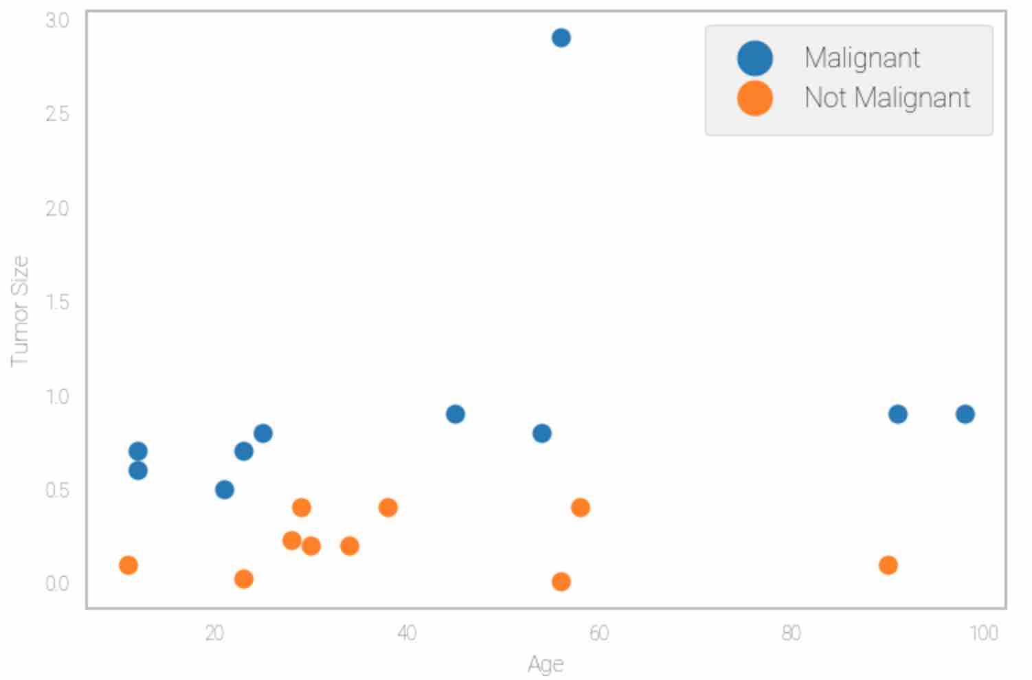
Next, let’s load a sample dataset. Download the dataset and upload to your Cloudera AI console. This is a text file with first column denoting age of person, second column denoting tumor size, and third column denoting if tumor is malignant or not.
Now, let’s treat the first two columns as X, the output variable y is the last column, and m denotes the number of training examples in the dataset.
datafile = 'Ages.txt'
cols = np.loadtxt(datafile,delimiter=',',usecols=(0,1,2),unpack=True)
X = np.transpose(np.array(cols[:-1]))
y = np.transpose(np.array(cols[-1:]))
m = y.size
X = np.insert(X,0,1,axis=1)
# Let’s divide the data based on class
malignant= np.array([X[i] for i in range(X.shape[0]) if y[i] == 1])
benign= np.array([X[i] for i in range(X.shape[0]) if y[i] == 0])
Next, plot the data to understand the distribution. The output should be similar to the figure below:
def plotData():
    fig = plt.figure()
    ax = fig.add_subplot(1, 1, 1)
    ax.patch.set_facecolor('white')
    ax.plot(malignant[:,1],malignant[:,2],'o',label="Malignant")
    ax.plot(benign[:,1],benign[:,2],'o',label="Not Malignant")
    ax.set_xlabel('Exam 1 score')
    ax.set_ylabel('Exam 2 score')
    ax.legend()
    ax.grid(False)

plotData()
Next, define the hypothesis function:
def sigmoid(z):
    return(1 / (1 + np.exp(-z)))
Next, define the cost function:
def costFunction(theta, X, y):
    m = y.size
    h = sigmoid(X.dot(theta))
    #J(beta)= -y log(ŷ)-(1-y)log(1-ŷ)
    J = -1*(1/m)*(np.log(h).T.dot(y)+np.log(1-h).T.dot(1-y))
    if np.isnan(J[0]):
        return(np.inf)
    return(J[0])
Next, define the gradient descent for optimization:
Gradient descent algorithm follows the below steps
1. Initialize the parameters
Repeat {
2. Make a prediction on y
3. Calculate cost function
4. Get gradient for cost function
5. Update parameters
}
def gradient(theta, X, y):
    m = y.size
    h = sigmoid(X.dot(theta.reshape(-1,1)))
    grad =(1/m)*X.T.dot(h-y)
    return(grad.flatten())
Initial parameter value theta is first given to the cost function and gradient descent algorithm to make further decisions on parameter values
initial_theta = np.zeros(X.shape[1])
cost = costFunction(initial_theta, X, y)
grad = gradient(initial_theta, X, y)
Next, use the minimize function to find the theta values that minimize cost:
from scipy.optimize import minimize
res = minimize(costFunction, initial_theta, args=(X,y), method=None, jac=gradient, options={'maxiter':400})
Next, define the predict function to make predictions
def predict(theta, X, threshold=0.5):
    p = sigmoid(X.dot(theta.T)) >= threshold
    return(p.astype('int'))
Next, you can now draw the logistic regression line which best classify the two classes with low cost as per the parameter values obtained using the gradient descent algorithm.
import matplotlib.pyplot as plt
plotData()
# Estimating the maximum boundary values of the graph
x1_min, x1_max = X[:,1].min(), X[:,1].max()
x2_min, x2_max = X[:,2].min(), X[:,2].max()
# defining the mesh grid for visualizing the plot
x_val, y_val = np.meshgrid(np.linspace(x1_min, x1_max), np.linspace(x2_min, x2_max))
# obtaining the parameter values to draw a line
h=sigmoid(np.c_[np.ones((x_val.ravel().shape[0],1)),x_val.ravel(), y_val.ravel()].dot(res.x))
h = h.reshape(x_val.shape)
# plot the line with the estimated parameter value h and the threshold as 0.5
plt.contour(x_val, y_val, h, [0.5], linewidths=1, colors='b')

Conclusion
Congratulations! You have learned the concepts behind building a logistic regression model using Python on Cloudera AI. You learned how to train logistic regression model using Python’s scikit-learn libraries. Hopefully, you had a chance to review the advanced section, where you learned to compute a cost function and implement a gradient descent algorithm.