Introduction
Making impactful predictions is one of the important skills that can help businesses grow. Suppose you were given a data scientist position to use census data to predict whether a person's annual income exceeds 50,000 dollars. You identify this as a classification problem, so you want to implement a classification model. In this tutorial, you will be introduced to a decision tree classification and a random forest models using Cloudera AI; an experience on Cloudera Platform. You will also learn about attribute selection measures, as well as how to optimize decision tree and random forest classification models and their respective advantages and disadvantages.
Prerequisites
To better understand this tutorial, you should have a basic knowledge of statistics and linear algebra.
You should have a Python 3 session set up in Cloudera AI before you start implementing the code.
Outline
Concepts behind Decision Tree and Random Forest models
Building decision tree and random forest models using scikit-learn on Cloudera AI
Conclusion
Concepts behind decision tree and random forest models
A decision tree helps in classifying examples by using a tree-like graph from root to a leaf node that holds the final answer for the current example. Each node in the tree is a feature in the dataset, and each edge in the tree descending from the node corresponds to one of the answers to the question asked. For example, let's assume you want to play badminton on a particular day: how will you decide whether to play or not? Let's say you go out and check to see, for example, if it is sunny, cloudy, or rainy. You take various factors into account to decide if you want to play or not. Suppose that you have collected data for the last week as shown below:
Day |
Weather |
Temperature |
Wind |
Humidity |
Play? |
1 |
sunny |
hot |
strong |
high |
no |
2 |
sunny |
hot |
weak |
high |
no |
3 |
cold |
low |
weak |
low |
play |
4 |
cold |
mild |
weak |
high |
play |
5 |
sunny |
mild |
weak |
low |
play |
6 |
cold |
low |
strong |
low |
no |
7 |
sunny |
hot |
weak |
high |
no |
Table 1: The table shows the sample data collected during a week, and this data includes the attributes day, weather, temperature, wind, humidity, and play. These attributes contribute to decision making when the model encounters unseen examples.
You have collected all the factors that are important for deciding whether you can play or not. Based on the data in Table1, you could make a decision. But what if you encounter a situation that is different from the available data. In such a case, a decision-tree trained model can help you include all the possible paths, allowing you to make the best decision. Decision trees are often used to answer this type of question: “Given a labeled dataset, how should we classify new samples?”
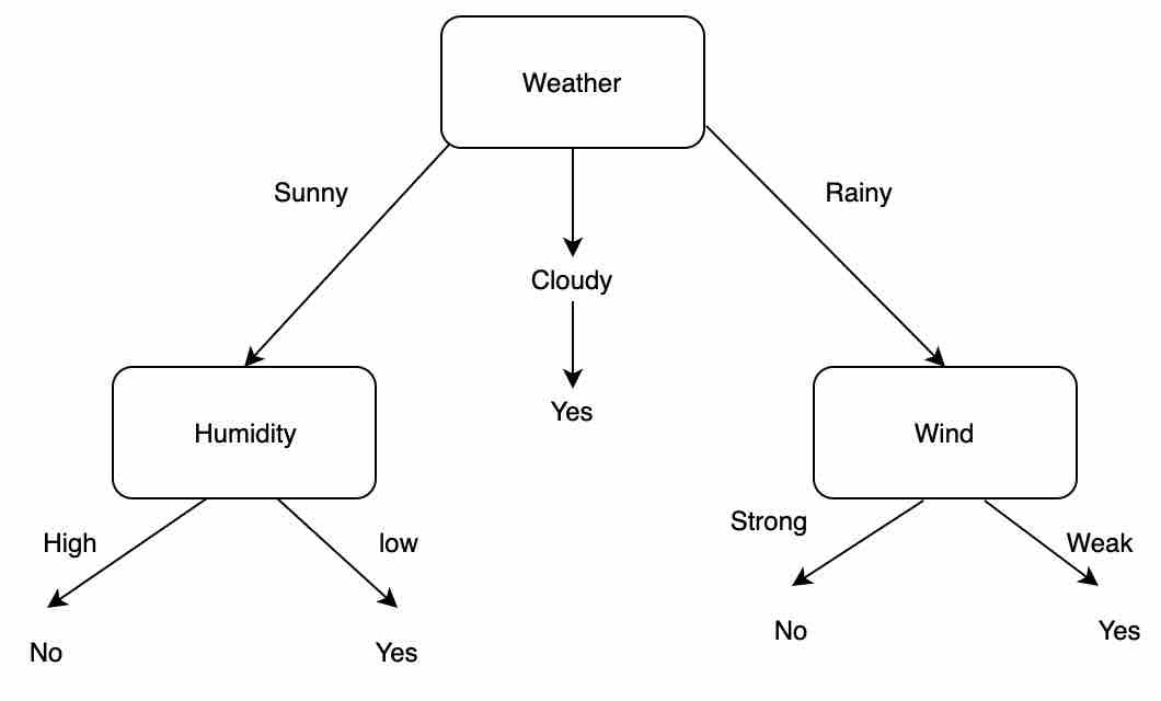
Figure 1: Sample data represented as a decision tree graph. An unseen example can use this decision tree knowledge to obtain a final classification result.
Decision tree algorithm
As you can observe in Figure 1, a decision tree is a flow chart structure where the topmost node is known as the root node, which learns to partition data on the basis of an attribute value. This process takes place recursively to find the best attribute to occupy the root node. All the internal nodes represent attributes in the dataset, each arrow represents a decision rule, and each leaf node represents the outcome. This representation of a decision tree makes the model easily interpretable.
Pseudo code for implementing a decision tree algorithm:
Select the best attribute as the root to split the data using best attribute selection measures
The selected attribute now becomes the decision node, which splits the data into smaller subsets
Build the tree recursively by repeating the above process until you find the leaf nodes in all the branches and no more attributes are left
Assumptions made while creating the decision tree model:
At the beginning of creating a decision tree, the entire training data is considered as the root
It is usually preferable that attribute values be categorical; if there are any continuous values, they are discretized prior to building a decision tree
All the examples in the data are distributed recursively, on the basis of attribute values
Selection of the root node and the internal nodes is made by using statistical attribute selection measures such as Gini index, Gain ratio, Information gain, etc.
Brief description of best attribute selection measures
Attribute selection measures help choose the best splitting criterion to partition data. Best score attribute is selected as the splitting attribute. Some of the most popular selection measures are Gini index, Gain ratio, and Information gain. Let’s understand the important concept of a splitting criterion below.
Entropy: Entropy refers to the randomness or impurity in a group of examples.
Information gain: Information gain computes the difference between entropy before a split and average entropy after a split in the dataset.
Gini ratio: One of the major drawbacks of using information gain is its bias toward the attribute with many outcomes. For example, if your data has an attribute named college_id that is unique, this attribute holds zero information gain because of pure partition. Thus, information gain seems to prefer attributes with a large number of distinct values. To handle this bias, an extension of information gain is made, known as the gain ratio. Gain ratio handles the issue of bias by normalizing the information gain. The attribute with the highest gain ratio is chosen as the splitting attribute.
Gini index: The Gini index is calculated by subtracting the sum of the squared probabilities of each class from one. For more information about attribute measures in detail, please look into construction of decision tree selection measures. Ultimately, you have to experiment with your data and the splitting criterion.
Advantages using a Decision Tree:
Easy to interpret to make decisions, based on the visualization of a tree
Decision trees can handle both numerical and categorical data
Extremely fast, and performs well on large datasets
Decision trees are robust to outliers
Disadvantages using a Decision Tree:
Decision trees are prone to overfitting, especially when a tree is deep
A decision tree can easily become unstable, meaning a slightly different sub-sample can cause the structure of the tree to change. It overfits by learning noise data as well, and optimizes for that particular sample, which causes its variable importance order to change significantly
A decision tree often involves more time to train the model
Calculations can become more complex when the number of class labels increases
Although the current generation of GPUs can handle them, training time might take a little longer
Random forest model
The random forest model gained importance in dealing with overfitting problem faced by decision trees. You may wonder why decision trees overfit: The objective of machine learning models is to generalize previously unseen data. In the case of decision trees, they can learn a training set to a point of high granularity that makes them easily overfit. Allowing a decision tree to split to a granular degree is the behavior of this model that makes it prone to learning every point extremely well — to the point of perfect classification — i.e., overfitting.
Several steps can be taken to ensure decision trees do not overfit to the data: 1) Reduce the complexity of a decision tree model by pruning it. This can be done in scikit-learn by using the max_depth parameter to control the complexity. 2) Check for class imbalance of data by making sure that enough data is available for each class in the dataset, so that the model is not biased toward one class.
Because decision trees are greedy and are also prone to finding locally optimal solutions without considering broader assumptions on data, one of the reasons ensemble models like the random forest model are ideal is because they generalize better. The random forest model allows for weighing different aspects of a decision tree with techniques like bootstrapping, random variable selection, and sample weight selection, and thus to generalize better.
Pseudo code of a random forest algorithm:
Random sub-sampling of data from a given dataset
Construct a decision tree for each data sample and predict the result from each decision tree
Predict the outcome using these decision trees
Calculate the vote for each of the targets predicted by each tree
The target with the highest vote is considered the final prediction of the random forest algorithm
Important hyperparameters:
n_estimators: Number of trees in the forest.
This is an optional parameter. You can instantiate the value of your choice. Usually the higher the number of trees, the higher the prediction accuracy. Default value for this parameter is 10.
criterion: Function to measure the quality of the split.
The default parameter is Gini. This parameter is tree specific.
max_features: Maximum number of features considered for the best split.
The default is “auto.” It will take all the features in a single run. Max_features=sqrt (n_features) takes the square root of the total number of features in a single run. Again, this is an optional parameter.
max_depth: Maximum depth or height of the tree.
The default is none: You can specify the depth to perform pruning of the tree and reduce the complexity, which helps to reduce overfitting. Again, this is an optional parameter.
min_samples_split: Minimum number of samples required in a leaf node before splitting. If the number of samples is greater than a threshold value, then the node is split. This is an optional parameter, with default value of 2.
min_samples_leaf: Minimum number of data points allowed in a leaf node. This is an optional parameter, with default value of 1.
random_state: Defines random selection to compare between different models. This parameter allows the model to obtain consistent results on re-run. This is an optional parameter, with default of none.
bootstrap: The method for sampling data points (with or without replacement).
Advantages using Random Forest:
The random forest algorithm can be used for both classification and regression.
A greater number of trees participating can prevent the overfitting of the model because the final decision is based on the predictions of multiple trees.
It can model for categorical values just like decision trees do.
You can learn relative feature importance, which helps in selecting the features that contribute the most as a classifier.
Disadvantages using Random Forest:
Random forests are slow in generating predictions because they are ensembles of multiple decision trees. Whenever a prediction is made, all the trees in the forest have to make a prediction for the same input, and then perform votes on it. This whole process is time-consuming.
The model is more difficult to interpret than a decision tree, where you can easily analyze a decision by following the path taken in that tree.
Building decision tree and random forest models using scikit-learn on Cloudera AI
Cloudera AI is a secure enterprise data science platform that enables data scientists to accelerate their workflow from exploration to production. Cloudera AI allows data scientists to utilize already existing skills and tools, such as Python, R, and Scala, to run computations in Hadoop clusters.
Cloudera AI allows you to run your code as a session or a job. A session is a way to interpret your code interactively, whereas a job allows you to execute your code as a batch process and can be scheduled to run recursively.
You can create your own project, in which you can set up your session required for this tutorial. You can follow the steps in Fig 2: provide your project name, and you can choose your project to be private or public, and then select the language of your choice. For this tutorial, you would select Python and click on Create Project. Enter the project you have created.
One of the interesting things about Cloudera AI is that you can also connect to a GitHub account directly and pull the code to execute on the workbench. Feel free to run your code snippets by connecting to your GitHub account.
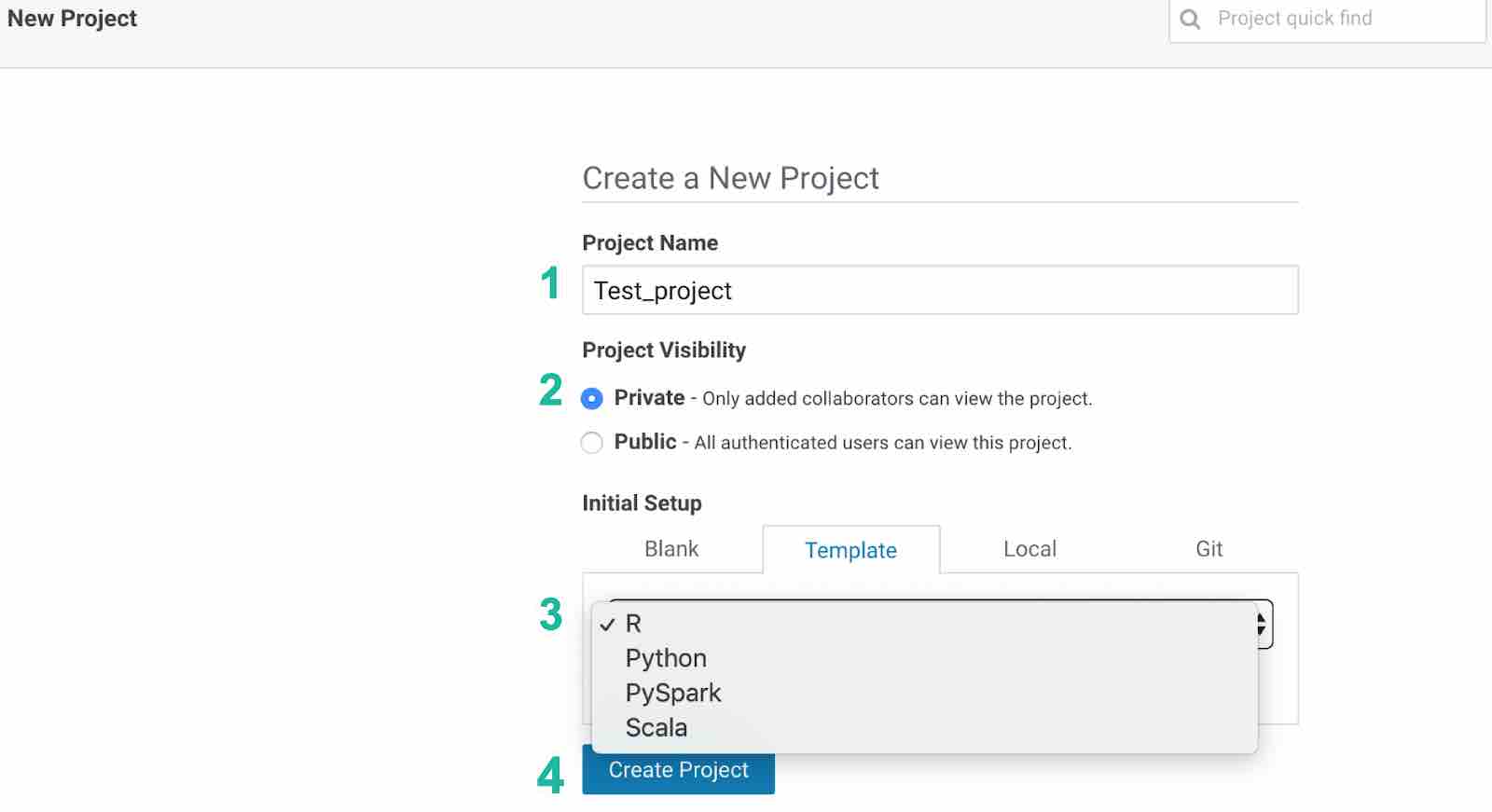
Figure 2: Steps to create your own project on Cloudera AI
In order for us to use the Python script needed for this tutorial, select a Python 3 engine with this resource allocation configuration:
2 vCPU
4 GB Memory
0 GPU (It's okay if you don't have any, but it's great to know you can have them.)
We can use either a Jupyter Notebook as our editor or a Workbench: feel free to choose your favorite.
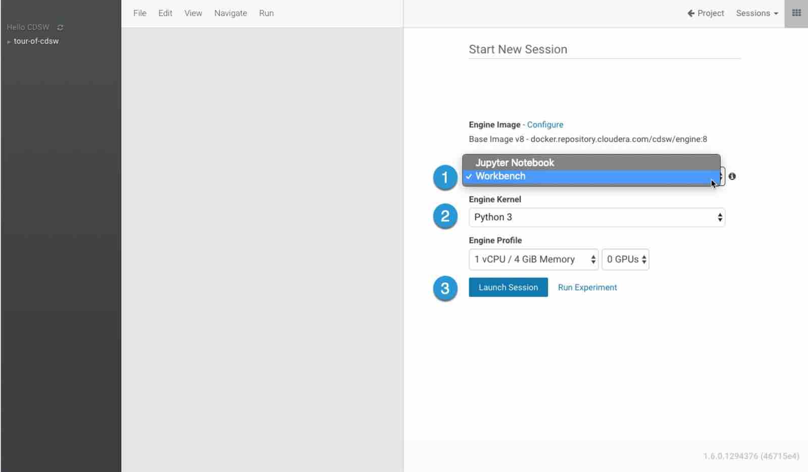
Figure 3: Steps to create Python session for running code snippets
Once you have the session open, copy and paste the code snippets you encounter by following this tutorial. You will be using the Adult dataset from University of California Irvine Machine Learning Repository to classify people based on their income. You can download this data and import the data files into your Cloudera AI project. In the project overview, you will find an option to upload files as highlighted in Figure 4. You will be using two files: adult.data (training data), adult.test (testing data). Upload these two files into Cloudera AI, and you are good to proceed further into the tutorial.
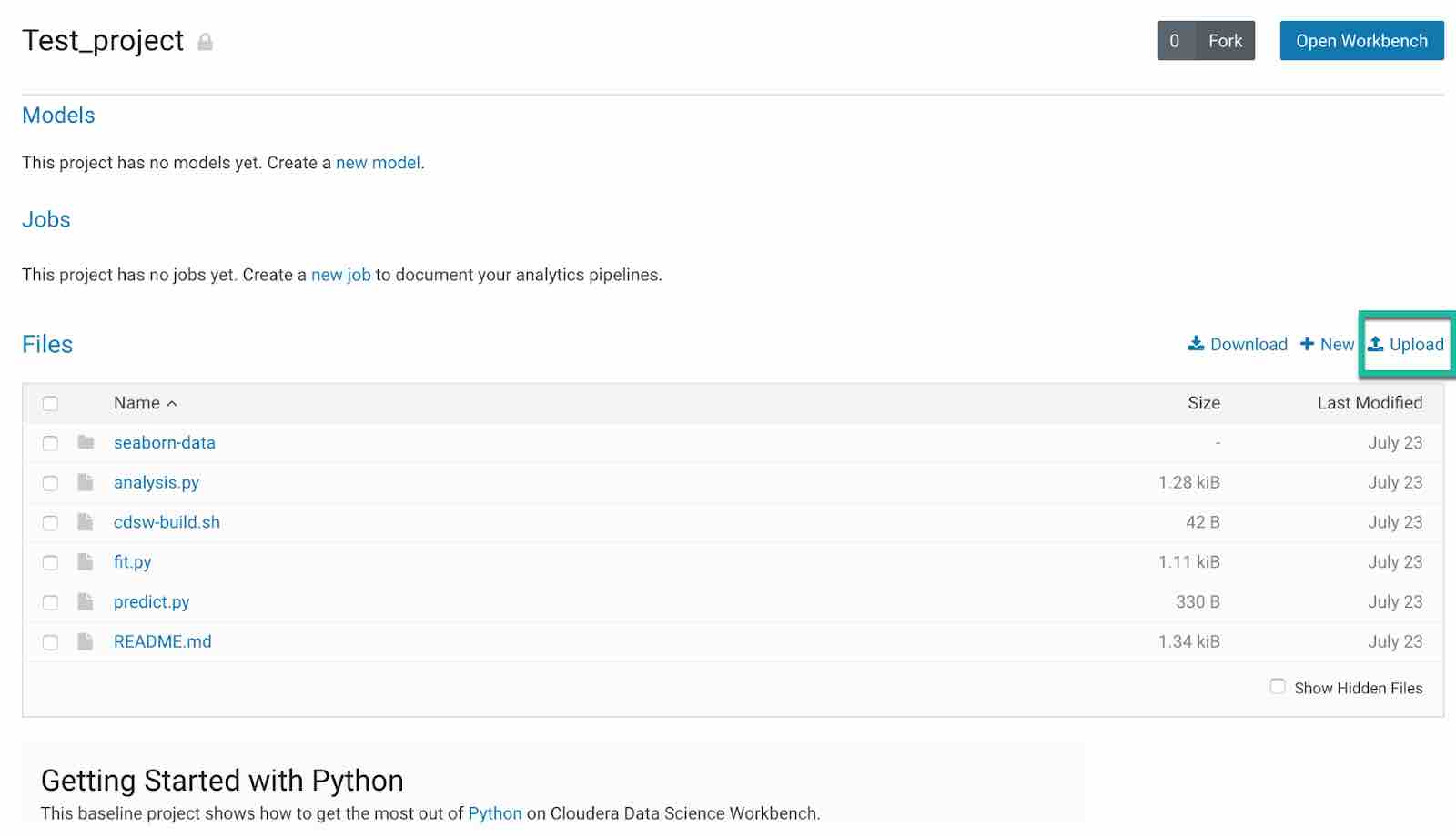
Figure 4: Figure highlights the upload option in your project to upload any files to your project in Cloudera AI
Dataset: University of California Machine Learning Repository: Adult Dataset
Dataset overview: This dataset consists of 14 attributes, and the data is used to predict whether income exceeds $50,000 per year, based on census data.
Import the dataset using pandas dataframe. Store the data into data frame called training_data.
import pandas as pd
training_data = pd.read_csv('adult.data', sep=',', names=['Age','Workclass','fnlwgt','Education','Education_Num','Martial_Status','Occupation','Relationship','Race','Sex','Capital_Gain','Capital_Loss','Hours_per_week','Country','Target'])
Next, check the correctness for the dataset by observing the first few rows of the dataset using head() command:
training_data.head()
Similarly, load the testing data into the pandas dataframe called testing_data:
testing_data = pd.read_csv('adult.test', names=['Age','Workclass','fnlwgt','Education','Education_Num','Martial_Status','Occupation','Relationship','Race','Sex','Capital_Gain','Capital_Loss','Hours_per_week','Country','Target'])
Next, check the correctness for the dataset by observing the first few rows of the dataset using head() command:
testing_data.head()
Encode the target variables to convert the problem into a binary classification problem:
testing_data = testing_data[(testing_data['Target'] == ' >50K.') | (testing_data['Target']==' <=50K.')]
# encode target variable as integer
training_data.loc[training_data['Target']==' <=50K', 'Target'] = 0
training_data.loc[training_data['Target']==' >50K', 'Target'] = 1

testing_data.loc[testing_data['Target']==' <=50K.', 'Target'] = 0
testing_data.loc[testing_data['Target']==' >50K.', 'Target'] = 1
Next, let’s perform a sanity check on the datatypes to fix any issues found.
First, test the training set data types:
training_data.dtypes
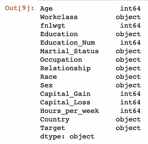
Next, check the data types of the test data:
testing_data.dtypes
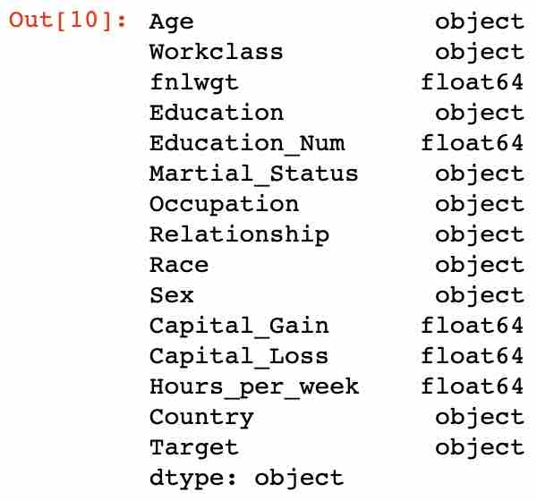
You can observe the difference in the data types of a few attributes compared to the training data. This often happens when you are dealing with raw data from source systems. Let’s go ahead and fix them:
testing_data['Age'] = testing_data['Age'].astype(int)
testing_data['fnlwgt'] = testing_data['fnlwgt'].astype(int)
testing_data['Education_Num'] = testing_data['Education_Num'].astype(int)
testing_data['Capital_Gain'] = testing_data['Capital_Gain'].astype(int)
testing_data['Capital_Loss'] = testing_data['Capital_Loss'].astype(int)
testing_data['Hours_per_week'] = testing_data['Hours_per_week'].astype(int)
Handling missing values: Here we are considering replacing missing values in categorical columns with the mode of the column and numerical columns with the mean of the column. We are taking this approach as this is a well-known stats approach that is widely used (instead of dropping missing values, which might lead to loss of data):
for c in training_data.columns:
    if training_data[c].dtype.name == 'object':
        training_data[c].fillna(training_data[c].mode()[0], inplace=True)
        testing_data[c].fillna(training_data[c].mode()[0], inplace=True)
    else:

        training_data[c].fillna(training_data[c].median(), inplace=True)
        testing_data[c].fillna(training_data[c].median(), inplace=True)
Let’s check the shape of both the training and the testing set:
training_data.shape, testing_data.shape

You can observe that there are 32561 training examples and 109 features in the training set, and 16281 examples and 108 features in the test set. As you can see, there is a difference between the number of features in the training and test datasets, and we need to address this issue to prevent any errors when making the predictions.
Let’s find the missing feature in our test dataset with the Python set method:
set(training_data.columns) - set(testing_data.columns)
Result: {'Country_ Holand-Netherlands'} seems to be the missing feature.
Add the missing data column and set it to zero:
testing_data['Country_ Holand-Netherlands'] = 0
Next, define the training and test dataset:
y_train = training_data['Target']

X_train = training_data.drop(["Target"],1)

y_test = testing_data['Target']

X_test = testing_data.drop(["Target"],1)
Next, build the decision tree classifier using scikit-learn:
from sklearn.tree import DecisionTreeClassifier
As an example, we are considering maximum depth max_depth of the tree to be 5 and random state value to be 17.
Note: These are just sample values that are considered reasonable. Feel free to experiment with different values.
tree = DecisionTreeClassifier(max_depth=5, random_state=17)
tree.fit(X_train, y_train)
Next, using the built classifier, predict the target using the test dataset:
tree_predictions = tree.predict(X_test)
Using the below commands, compute the accuracy score:
from sklearn.metrics import accuracy_score
accuracy_score(y_test, tree_predictions)
Hyperparameter tuning: Parameters that define the model architecture are referred to as hyperparameters, and thus this process of searching for the ideal model architecture is referred to as hyperparameter tuning. It is possible, and recommended, to search the hyperparameter space for the best cross validation score. GridSearchCV exhaustively considers all parameter combinations and retains the best combination.
Hyperparameter search using grid search cross validation:
from sklearn.model_selection import GridSearchCV
Here we are only giving the maximum depth parameter to be grid searched between the values 2 and 11. This search returns locally best tree parameters:
tree_params = {'max_depth': range(2, 11)}
locally_best_tree = GridSearchCV(DecisionTreeClassifier(random_state=17),
                                 tree_params)

locally_best_tree.fit(X_train, y_train)
Next, print out the best parameter value obtained:
print("Best parameters:", locally_best_tree.best_params_)
Result: Best params: {'max_depth': 9}
Finally, using the parameters maximum depth set to 9 and random state value set to 17, we have an 84% predictive model accuracy.
tuned_tree = DecisionTreeClassifier(max_depth=9, random_state=17)
tuned_tree.fit(X_train, y_train)
tuned_tree_predictions = tuned_tree.predict(X_test)
accuracy_score(y_test, tuned_tree_predictions)
Result: 0.8481665745347338
Applying a random forest model to census data
As you have already learned using the decision tree model on census data, now let’s apply a random forest model to the same data and observe the accuracy of the model.
First, import the RandomForestClassifier from scikit-learn:
from sklearn.ensemble import RandomForestClassifier
For this exercise, you will be using the number of estimators as 100 and the random state value as 17. Feel free to experiment with other values.
rf = RandomForestClassifier(n_estimators=100, random_state=17)
Using the same training and testing dataset as in decision trees, fit the data to the random forest model:
rf.fit(X_train, y_train)
Let’s observe the accuracy scores with cross validation score as 3:
from sklearn.model_selection import cross_val_score
cv_scores = cross_val_score(rf, X_train, y_train, cv=3)
cv_scores, cv_scores.mean()
Let’s now predict with test data:
forest_predictions = rf.predict(X_test)
accuracy_score(y_test,forest_predictions)
As we have utilized GridSearch cross validation (GridSearchCV) in the case of decision trees, let’s apply the same function to obtain the best parameters. For the random forest model in this exercise, we are using maximum depth range values between 10 and 16.
forest_params = {'max_depth': range(10, 16)}
Use GridSearchCV to find the best parameters. Here we are using the number of estimators as 100, the random state value as 17, and the cross validation score as 3. Feel free to experiment with different values and observe the change in accuracy.
locally_best_forest = GridSearchCV(
    RandomForestClassifier(n_estimators=100, random_state=17),
    forest_params, cv=3, verbose=1)

locally_best_forest.fit(X_train, y_train)
Print the best parameter values obtained using GridSearchCV:
print("Best params:", locally_best_forest.best_params_)
Result: Best params: {'max_depth': 13, 'max_features': 45}
Now, predict the results using the test set:
tuned_forest_predictions = locally_best_forest.predict(X_test)
accuracy_score(y_test,tuned_forest_predictions)
Result: 0.8602051471039862
Finally, maximum depth set to 13 (value obtained as best parameter value for max_depth earlier) and random state value set to 17, we have an 86% predictive model accuracy.
As you have observed with the same maximum depth range as parameters to both the decision trees and random forest, you have seen an improvement in the model accuracy from 84% to 86% by using a random forest model. With further experimentation with the hyperparameters, you should be able to obtain an even higher random forest accuracy.
Conclusion
Congratulations! You have learned the concepts behind building decision tree models and random forest models using Python on Cloudera AI. We’ve written sample code on Cloudera AI and analyzed key hyperparameters affecting decision tree and random forest model performance.

