Introduction to convolutional neural networks
Introduction
In this tutorial, you will gain an understanding of convolutional neural networks (CNNs), a class of deep, feed-forward artificial neural networks that are applied to analyzing visual imagery. This tutorial will focus on the highlights of how you can use CNNs to deal with complex data such as images. It will also help you understand how convolutional neural networks have evolved over time, how CNNs have succeeded in the image-recognition space, and some of the underlying mathematics for the building blocks of the model. By the end of this tutorial, you should have a set of tools for building your own CNN model.
Prerequisites
Basic knowledge of neural networks
Knowledge of Python to understand code snippets
Outline
Convolution neural networks essentials
What are convolution neural networks
Convolutional neural networks are a class of deep neural networks that have gained in importance for visual recognition and classification. The architecture of these networks was loosely inspired by our brain, where several groups of neurons communicate with each other to provide responses to various inputs. Though the work with CNNs began in the early 1980s, they have recently become more popular as a result of significant technology advancements and computational capabilities that have allowed them to process large amounts of data and leverage the power of highly sophisticated algorithms in a much more reasonable amount of time.
How convolution neural networks are different from regular neural networks
In regular deep neural networks, you can observe a single vector input that is passed through a series of hidden layers. Each hidden layer is made up of a set of neurons that are connected to the previous layers, and is then connected to the output layer, which results in determining the class scores. It is always a challenge to deal with image data due to its complexity. A model should have the capability to scale well.
For example, if you consider an image with size 64x64x3 (height, width, color channels), then the total number of input features is 12288, and if your first hidden layer contains 100 units it results in a 12288x100 = 1228800 weight matrix, which a regular neural network can still handle. However, for high resolution images, for example 1000x1000x3, the number of input features will be 3 million, and with 1000 neurons in your hidden layer, you will have a 3 billion weight matrix, which is huge and expensive to compute. To deal with this kind of scenario, a convolution operation is introduced.
How convolution operation works
Images are seen by a machine as a matrix of pixel values. One of the important tasks of a convolution layer is to detect edges in an image. For example, see Fig 1, where a kernel is applied to an image to detect vertical edges. A convolution operation helps to detect the edges. Instead of handpicking the kernel values, the convolution layer tries to select the parameter values that are best suited to detecting the vertical and horizontal edges.
 .
. 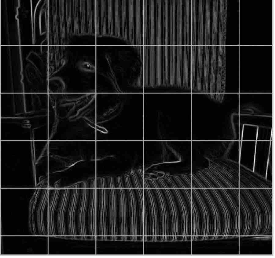
Fig 1: Horizontal edge detection by the initial convolution layers of the model
When a convolution layer receives the input, a filter is applied to the images and is multiplied by the corresponding kernel values to give the output as a scalar output value. For example, see Fig 2, which shows a 3x3 filter and is mapped onto a few pixels on the image as shown on the left, and then the dot product is performed this way: 134x0+134x-1+117x0+153x-1+144x5+141x-1+152x0+154x-1+150x0 = 138). The entire image is scanned in this manner, using the filter to obtain the convolution computation matrix.
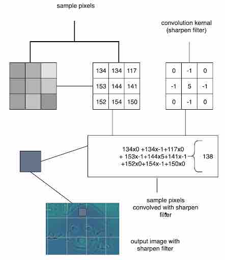
Fig 2: Convolution operation performed on a section of image using 3x3 filter
The same operation is performed on Red, Green, and Blue channels, which gives rise to three convolution outputs. Thus the input to the next layers will be this volume of data.
Techniques used in performing convolutions:
Two of the common techniques used when applying convolution to the image are padding and striding.
Padding: While performing convolutions using kernel, we can observe that the corners of the image are covered only once, whereas the other pixels in the middle are covered at least twice. Essentially the edges are trimmed off, not given much attention. Hence you are missing the data at the edges of the image, and this may lead to poor training of your model. Padding is a technique used to solve this problem by adding a layer of 0 “fake” pixels around your image. With padding, you preserve the original dimensions of your image. Fig 3 gives you an idea of how it works.
Fig 3: Filter sliding on to the padded image , Source: theano_convolution_arithmetic
Stride: Stride is a technique where you skip some of the slide locations. A stride 2 is to skip slide by a factor of two. This helps in reduction of the output size when compared to input size. Fig 4 illustrates a stride factor of 2.
Fig 4: Stride=2 operation performed by the filter, Source: theano_convolution_arithmetic
Layers used to build Convolution Neural Networks
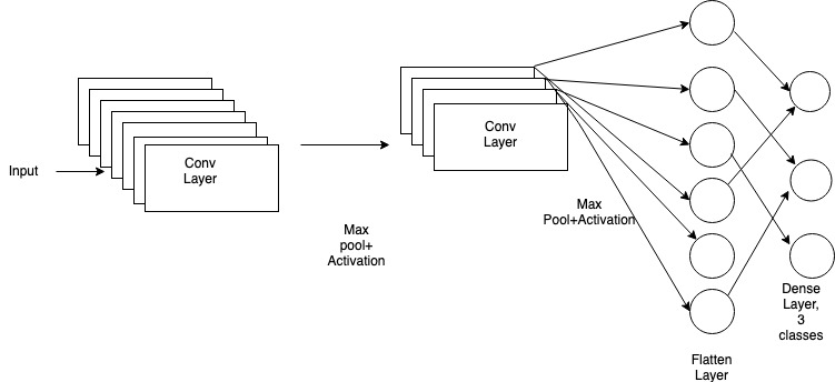
Fig 5: Example of Layers built in a CNNetwork model
Layers used to build convolutional neural networks
In this section we will cover basic layers used to build a CNN model. For complete implementation in building a convolutional neural network, check out the Further Reading section.
Review the pseudo code below to see how layers can be added to a sequential model using Keras. Conventionally, many of the algorithms follow the order Convolution Layer- Max Pooling Layer- Dense Layer.
The Input Layer is the first layer, which takes in input shape as a parameter, followed by convolution layers with parameters like number of filters, kernel size, padding in general.
model = Sequential()
model.add(Conv2D(6, (3, 3), padding='same',
                 input_shape=(32,32,3))
Activation function will deal with the nonlinearity of the data and send data to the next layer.
model.add(Activation('relu'))
You can add convolution layers specifying your own parameters: here, 16 refers to the number of filters and (3,3) refers to kernel size.
model.add(Conv2D(16, (3, 3)))
model.add(Activation('relu'))
Max Pooling layer can then be used after the convolution layer, which helps reduce the dimension of data.
model.add(MaxPooling2D(pool_size=(2, 2)))
Flatten layer can be used to convert the data into single dimension vector to pass it to Dense Layer, which is a feed-forward neural network.
model.add(Flatten())
Dense Layer is responsible for predicting the output. The value 10 specifies the number of classes to predict scores. Softmax, the final layer of a neural network, is used to calculate the class probabilistic scores.
model.add(Dense(10))
model.add(Activation('softmax'))
Let’s look into each layer in detail:
Input Layer: This is the layer that takes in the image with its dimensions of height, width, and its three channels of Red, Green, and Blue values for a color image, or one channel for a grayscale image.
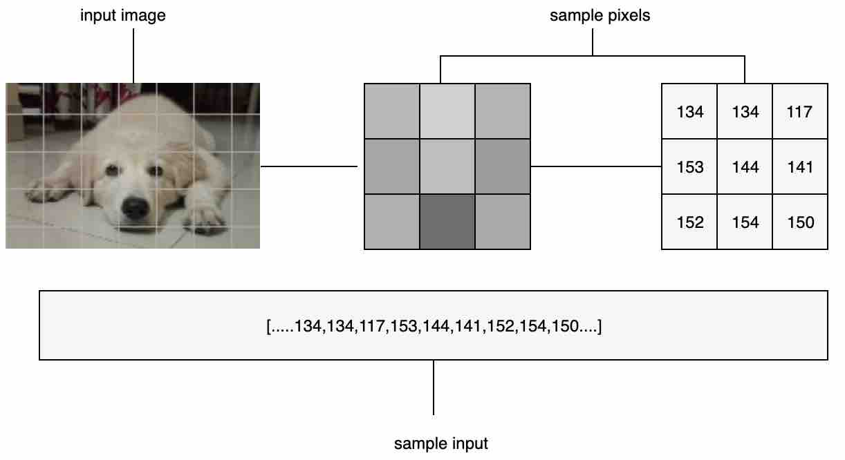
Fig 6: Input image transformed as an input vector to feed the model
Convolution Layer: This layer contains neurons to perform convolution operations on the input, each performing a dot product between the input volume connected and their weights. Two important things to understand about the importance of this layer compared to a regular neural networks are that it allows parameter sharing and sparse connection. Consider the example of the edge detector, where you can use the same kernel parameters that are learned once but can be applied to the entire image. This decreases the overhead involved in calculating parameters every time. Also, in each layer the output value depends on only a small number of inputs. The convolution layer is also good at translation invariance, which means even though the image is shifted, it can still recognize object identity.
Pooling Layer: The objective of this layer is to down-sample an input representation, reducing its dimensionality. The purpose of this is to help prevent overfitting, as well as reducing the computation cost. The pooling layer has no parameters to learn. The backpropagation algorithm doesn't use any parameters of the max pooling layer to learn, hence it is a static function that won’t add overhead in your deep neural networks. Commonly used hyperparameters for this layer are the number of filters, strides, the number of channels, and the type of pooling (max or average). Padding is mostly not used when performing pooling. Max pooling is done by applying a max filter to non-overlapping subregions of the initial representation.
Consider an input with 32x32x1 (NhxNwxNc) passed into the max pool layer with filters as 2 (f), strides as 2 (s): the output of this layer would be ((Nh-f)/s+1, (Nw-f)/s+1, Nc) = (16,16,1). Fig 8 shows the application of the max pool layer applied to 4x4x1 input with 2x2 filter and stride as 2 to get 2x2 output, each filter applied on the input, returning the max of the pool. You can also apply average pooling for the same example, which gives the result as the average of the pool (which is not as often used in real life, as compared to max pool). The significance of using max pool is that it captures a strong intuition of what you are looking for. For example, if you want to identify a cat in your image, max pooling will try to capture mostly the region where the cat can reside in the image, rather than focusing on the other parts of the image.
You can also use the same parameters for more than one channel input, and it will create outputs for all three channels independently.
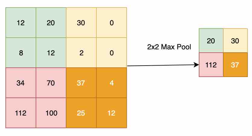
Fig 7: 2x2 max pool operation performed on the convolution layer output
Dropout Layer: It is often the case that deep neural networks overfit the data. The dropout layer acts as a good regularizer by dropping out a few nodes during the training. It corrects the situation where the network layer tries to co-adapt its mistakes from the previous layer and creates problems of overfitting. The dropout layer takes a probabilistic approach for dropping the nodes, which can be passed as a parameter to the dropout function.
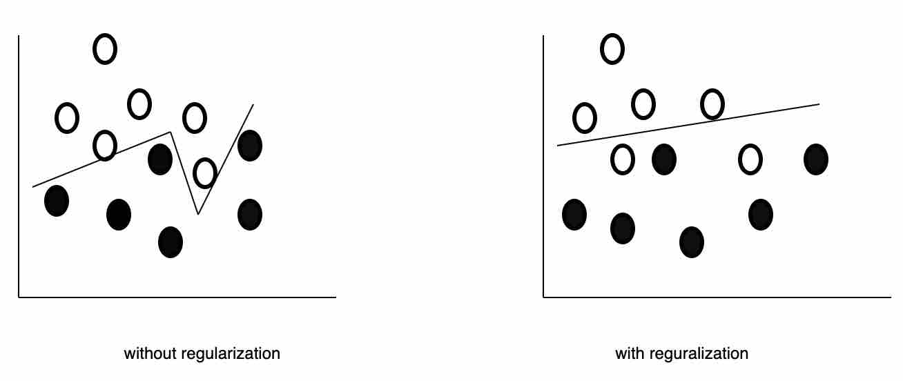
Fig 8: Without regularization can lead to overfitting, which tends to fit the training data perfectly but makes many mistakes on the actual testing data
Flatten Layer: After the pooling layer is done with its operation, the model will have a pooled feature map. This layer flattens the pooled feature map to a single column to pass it to the “fully connected layer,” which is like an artificial neural network, to produce the output.
Fully Connected Layer: Neurons in a fully connected layer have full connections to all activations in the previous layer, as seen in regular neural networks. The main difference between the convolution layer and the fully connected layer is that convolution layers are connected to the local regions and the neurons share parameters.
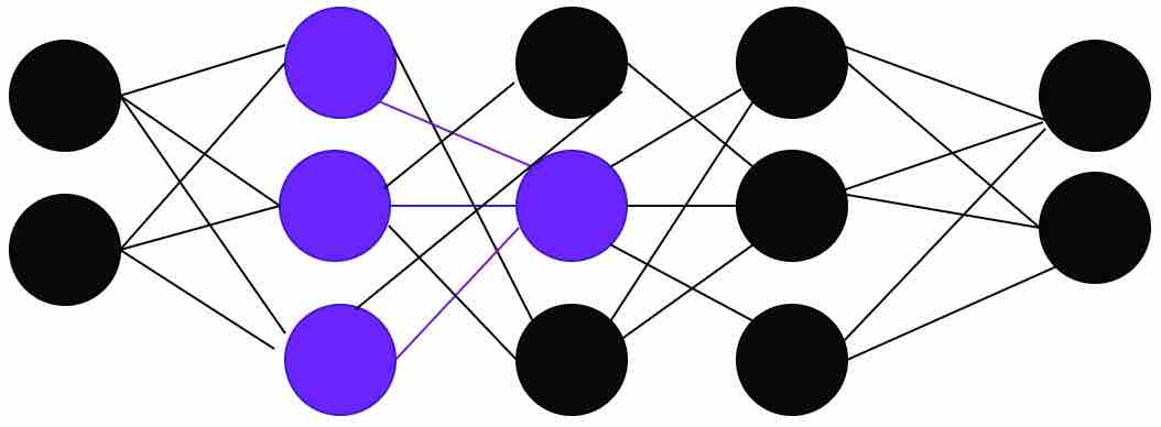
Fig 9: Fully connected neural network
Activation Functions:
The main purpose of the activation functions is to deal with nonlinearity. Without this, a neural network would be just a linear regression model. For CNN to learn from higher-dimension data such as images, audio, or video, it has to deal with nonlinearity. Activation functions should also be differentiable so as to perform backpropagation in learning the weights.
These are three of the most commonly used activation functions:
- Sigmoid or logistic
- Tanh
- RELU(Rectified Linear Units)
Sigmoid or Logistic: This function is of the form f(x) = 1 / 1 + exp(-x)and ranges between 0 and 1. It is not used much these days, due to the vanishing gradient problem, and it’s known to have slow convergence. The output of this function is also not 0-centered, hence optimization is difficult because the gradient updates tend to go far in directions.
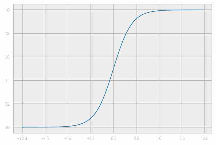
Fig 10: Representation of sigmoid function
Tanh: The activation function is f(x) = 1 — exp(-2x) / 1 + exp(-2x), the range is between -1 and 1. The output of this function is centered to 0, hence the optimization is better compared to sigmoid, but it still suffers from the vanishing gradient problem.
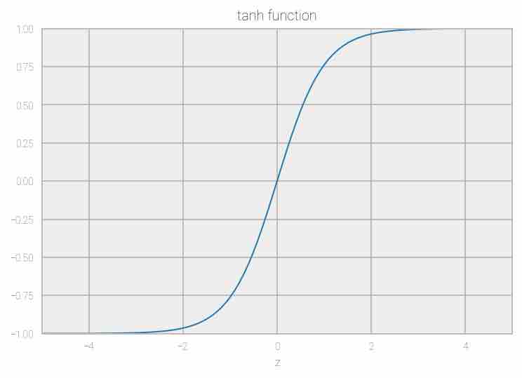
Fig 11: Representation of tanh function
ReLU( Rectified Linear Units): This works on the following rule: R(x) = max(0,x). For example, if x < 0, R(x) = 0, and if x >= 0, R(x) = x. It is very simple and efficient in converging and is widely used in most state-of-the-art architectures. It is known to solve the vanishing gradient problem.
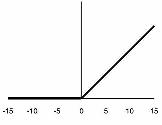
Fig 12: Representation of ReLU function
For output layers, the softmax function is used to calculate the probabilities of the class to which an object belongs in an object classification use case. For a regression problem, you can use regression at your output.
Though ReLU performs well, leaky ReLU was introduced to fix a drawback of ReLU where sometimes nodes become fragile and die—a gradient update on the node is not activated, which results in dead neurons. Leaky ReLU introduces a slope to keep updates live.
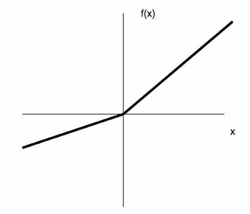
Fig 13: Representation of leaky ReLU function
Data Augmentation: This is a technique that is used to reduce overfitting—thanks to CNN, which has the capability of translation invariance studied earlier.
Use cases
- To make driving decisions in self-driving cars
- To detect a tumor/lesion in a patient's body with a CNN classification model
- Using semantic image search to obtain all the similar images from your database
- To classify galaxies, train multiple models, and then print some of the hidden layers to get a glimpse of how the neurons are learning
- To process insurance claims by identifying the damage based on the images
- To use CNN for image captioning
Further reading
Convnet Playground: An interactive CNN playground to accompany the Cloudera Deep Learning for Image Analysis report. It allows you to perform semantic image search using CNN and model interpretability.